Unveiling the Power of Quantile Plots for Data Visualization
Explore the significant role of quantile plots in displaying ordered values against ranks or probabilities. Delve into their historical significance, usage in Stata, and related plot variations for effective data analysis. Gain insights into why quantile plots remain a preferred choice for visualizing univariate distributions.

Download Presentation

Please find below an Image/Link to download the presentation.
The content on the website is provided AS IS for your information and personal use only. It may not be sold, licensed, or shared on other websites without obtaining consent from the author. Download presentation by click this link. If you encounter any issues during the download, it is possible that the publisher has removed the file from their server.
E N D
Presentation Transcript
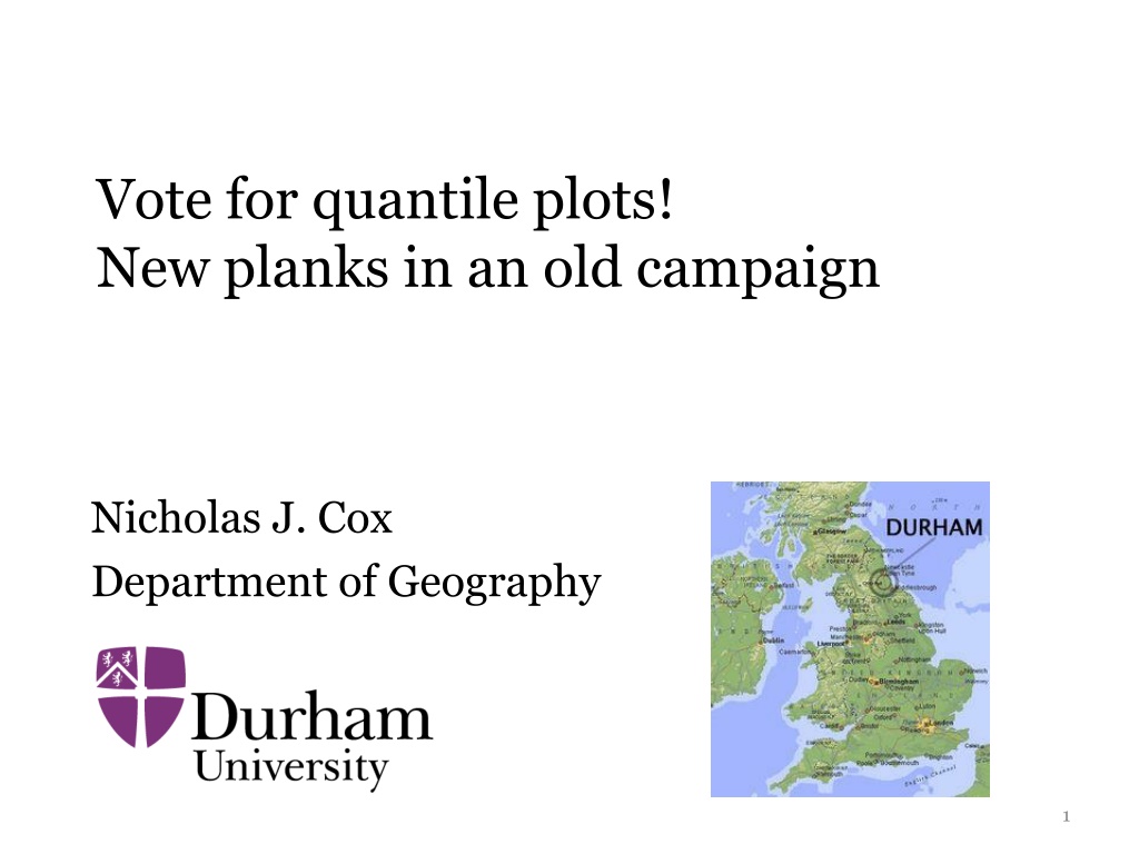
Vote for quantile plots! New planks in an old campaign Nicholas J. Cox Department of Geography 1
Quantile plots Quantile plots show ordered values (raw data, estimates, residuals, whatever) against rank or cumulative probability or a one-to-one function of the same. Tied values are assigned distinct ranks or probabilities. 2
Example with auto dataset 40 Quantiles of Mileage (mpg) 30 20 10 0 .25 .5 .75 1 Fraction of the data 3
quantile default In this default from the official command quantile, ordered values are plotted on the y axis and the fraction of the data (cumulative probability) on the x axis. Quantiles (order statistics) are plotted against plotting position (i 0.5)/n for rank i and sample size n. Syntax was sysuse auto, clear quantile mpg, aspect(1) 4
Quantile plots have a long history Adolphe Quetelet Sir Francis Galton G. Udny Yule Sir Ronald Fisher 1796 1874 1822 1911 1871 1951 1890 1962 all used quantile plots avant la lettre. In geomorphology, hypsometric curves for showing altitude distributions are a long-established device with the same flavour. 5
Quantile plots named as such Martin B. Wilk Ramanathan Gnanadesikan 1922 2013 1932 2015 Wilk, M. B. and Gnanadesikan, R. 1968. Probability plotting methods for the analysis of data. Biometrika 55: 1 17. 6
A relatively long history in Stata Stata/Graphics User's Guide (August 1985) included do-files quantile.do and qqplot.do. Graph.Kit (February 1986) included commands quantile, qqplot and qnorm. Thanks to Pat Branton of StataCorp for this history. 7
Related plots use the same information Cumulative distribution plots show cumulative probability on the y axis. Survival function plots show the complementary probability. Clearly, axes can be exchanged or reflected. distplot (Stata Journal ) supports both. Many people will already know about sts graph. 8
So, why any fuss? The presentation is built on a long-considered view that quantile plots are the best single plot for univariate distributions. No other kind of plot shows so many features so well across a range of sample sizes with so few arbitrary decisions. Example: Histograms require binning choices. Example: Density plots require kernel choices. Example: Box plots often leave out too much. 9
Whats in a name? QQ-plots Talk of quantile-quantile (Q-Q or QQ-) plots is also common. As discussed here, all quantile plots are also QQ-plots. The default quantile plot is just a plot of values against the quantiles of a standard uniform or rectangular distribution. 10
NJC commands The main commands I have introduced in this territory are quantil2 (Stata Technical Bulletin) qplot (Stata Journal) stripplot (SSC) Others will be mentioned later. 12
quantil2 This command published in Stata Technical Bulletin 51: 16 18 (1999) generalized quantile: One or more variables may be plotted. Sort order may be reversed. by() option is supported. Plotting position is generalised to (i a) /(n 2a + 1): compare a = 0.5 or (i 0.5)/n wired into quantile. 13
A now bizarre detail The truncated name quantil2 was enforced by the 8.3 filename.ext restriction of MS-DOS so that no Stata command defined by an .ado could have a name longer than 8 characters. 14
qplot The command quantil2 was renamed qplot and further revised in Stata Journal 5: 442 460 and 471 (2005), with later updates: over() option is also supported. Ranks may be plotted as well as plotting positions. The x axis scale may be transformed on the fly. recast() to other twoway types is supported. 15
stripplot The command stripplot on SSC started under Stata 6 as onewayplot in 1999 as an alternative to graph, oneway and has morphed into (roughly) a superset of the official command dotplot. It is mentioned here because of its general support for quantile plots as one style and its specific support for quantile-box plots, on which more shortly. 16
Comparing two groups is basic superimposed juxtaposed 40 40 quantiles of Mileage (mpg) 30 30 Mileage (mpg) 20 20 10 0 .2 .4 .6 .8 1 10 fraction of the data Domestic Foreign Domestic Foreign Car type 18
Syntax was qplot mpg, over(foreign) aspect(1) stripplot mpg, over(foreign) cumulative centre vertical aspect(1) 40 40 quantiles of Mileage (mpg) 30 30 Mileage (mpg) 20 20 10 10 0 .2 .4 .6 .8 1 Domestic Foreign fraction of the data Car type Domestic Foreign 19
Quantiles and transformations commute In essence, transformed quantiles and quantiles of transformed data are one and the same, with easy exceptions such as reciprocals reversing order. So, quantile plots mesh easily with transformations, such as thinking on logarithmic scale. For the latter, we just add simple syntax such as ysc(log). Note that this is not true of (e.g.) histograms, box plots or density plots, which need re-drawing. 20
The shift is multiplicative, not additive? 40 40 30 30 quantiles of Mileage (mpg) Mileage (mpg) 20 20 10 10 0 .2 .4 .6 .8 1 fraction of the data Domestic Foreign Car type Domestic Foreign 21
multqplot (Stata Journal) multqplot is a convenience command to plot several quantile plots at once. It has uses in data screening and reporting. It might prove more illuminating than the tables of descriptive statistics ritual in various professions. We use here the Chapman data from Dixon, W. J. and Massey, F.J. 1983. Introduction to Statistical Analysis. 4th ed. New York: McGraw Hill. 22
age (years) systolic blood pressure (mm Hg) diastolic blood pressure (mm Hg) 70 190 112 52 90 80 42 130 75 120 33 110 23 90 55 0 .25 .5 .75 1 0 .25 .5 .75 1 0 .25 .5 .75 1 cholesterol (mg/dl) height (in) weight (lb) 520 74 262 70 331 68 180 67 276 163 245.5 147 135 62 108 0 .25 .5 .75 1 0 .25 .5 .75 1 0 .25 .5 .75 1 23
multqplot details By default the minimum, lower quartile, median, upper quartile and maximum are labelled on the y axis so we are half-way to showing a box plot too. By default also variable labels (or names) appear at the top. More at Stata Journal 12:549 561 (2012) and 13:640 666 (2013). 24
Raw or smoothed? Quantile plots show the data as they come: we get to see outliers, grouping, gaps and other quirks of the data, as well as location, scale and general shape. But sometimes the details are just noise or fine structure we do not care about. Once you register that values of mpg in the auto data are all reported as integers, you want to set that aside. You can smooth quantiles, notably using the Harrell and Davis method, which turns out to be bootstrapping in disguise. hdquantile (SSC) offers the calculation. 26
The reference Harrell, F.E. and Davis, C.E. 1982. A new distribution-free quantile estimator. Biometrika 69: 635 640. 27
Some results 40 H-D quantiles of mpg 30 20 10 0 .2 .4 .6 .8 1 fraction of the data Domestic Foreign 28
More could be said Some questions on the mpg example: Is the shift closer to multiplicative than additive? Would reciprocals be better, e.g. gallons per mile? Either way, quantile plots offer tools to precede or advise modelling of the data. 29
Fitting or testing named distributions Using quantile plots to compare data with named distributions is common. The leading example is using the normal (Gaussian) as reference distribution. Indeed, many statistical people first meet quantile plots as such normal probability plots. 31
Normal QQ-plots are a reasonable default Yudi Pawitan in his 2001 book In All Likelihood (Oxford University Press) advocates normal QQ-plots as making sense even when comparison with normal distributions is not the goal. 32
qnorm available but limited qnorm is already available as an official command but it is limited to the plotting of just one set of values. 33
Named distributions with qplot qplot has a general trscale() option to transform the x axis scale that otherwise would show plotting positions or ranks. For normal distributions, the syntax is just to add trscale(invnormal(@)) to scale plotting positions. @ is a placeholder for what would otherwise be plotted. invnormal() is Stata s name for the normal quantile function (as an inverse cumulative distribution function). 34
40 quantiles of Mileage (mpg) 30 20 10 -2 -1 0 1 2 invnormal(P) Domestic Foreign 35
A standard plot in support of t tests? This plot is suggested as a standard for two-group comparisons: We see all the data, including outliers or other problems. Use of a normal probability scale shows how far that assumption (read: ideal condition) is satisfied. The vertical position of each group tells us about location, specifically means. The slope or tilt of each group tells us about scale, specifically standard deviations. It is helpful even if we eventually use Wilcoxon-Mann- Whitney or something else. 36
What if you had paired values? Plot the differences, naturally. Nothing stops you plotting the original values too, but at some point the graphics should respect the pairing. 37
Different axis labelling? The last plot used a scale of standard normal deviates or z scores. Some might prefer different labelling, e.g. % points. mylabels (SSC) is a helper command, which puts the mapping in a local macro for your main command: mylabels 1 2 5 10(20)90 95 98 99, myscale(invnormal(@/100)) local(plabels) 38
Foreign Domestic 40 quantiles of Mileage (mpg) 30 20 10 1 2 5 10 30 50 70 90 95 9899 exceedance probability (%) 39
Syntax for that example sysuse auto, clear mylabels 1 2 5 10(20)90 95 98 99, myscale(invnormal(@/100)) local(plabels) qplot mpg, over(foreign) trscale(invnormal(@)) aspect(1) xla(`plabels') xtitle(exceedance probability (%)) xsc(titlegap(*5)) legend(pos(11) ring(0) order(2 1) col(1)) 40
Other named distributions? There are many, many named distributions for which customised QQ-plot commands could be written. I am guilty of programs for beta, Dagum, Dirichlet , exponential, gamma, generalized beta (second kind), Gumbel, inverse gamma, inverse Gaussian, lognormal, Singh-Maddala and Weibull distributions. But a better approach when feasible is to allow a distribution to be specified on the fly. 41
Harold Jeffreys suggested that error distributions are more like t distributions with 7 df than like Gaussians. 1939/1948/1961. Theory of probability. Oxford University Press. Ch.5.7 Sir Harold Jeffreys 1891 1989 1938. The law of error and the combination of observations. Philosophical Transactions of the Royal Society, Series A 237: 231 271 County Durham man established that the Earth s core is liquid pioneer Bayesian 42
plotted for probability in [0.001, 0.999] 6 4 2 kurtosis 5 t 0 7 df -2 -4 -6 -3 -2 -1 0 1 2 3 normal kurtosis 3 43
How to explore? Simulate with rt(7,) and samples of desired size. trscale(invt(7, @)) sets up x axis scale on the fly. 44
1 2 3 5 0 -5 4 5 6 5 quantiles of t7 0 -5 7 8 9 5 0 -5 -2 0 2 4 normal deviates -2 0 2 4 -2 0 2 4 45
1 2 3 5 0 -5 4 5 6 5 quantiles of t7 0 -5 7 8 9 5 0 -5 -4 -2 0 2 4 -4 -2 0 2 4 -4 -2 0 2 4 t with 7 df 46
Adding a box plot flavour Earlier we saw how extremes and quartiles could be made explicit on the y axis of a quantile plot. They are the minimal ingredients for a box plot. age (years) systolic blood pressure (mm Hg) diastolic blood pressure (mm Hg) 70 190 112 52 90 80 42 130 75 120 33 110 23 90 55 0 .25 .5 .75 1 0 .25 .5 .75 1 0 .25 .5 .75 1 cholesterol (mg/dl) height (in) weight (lb) 520 74 262 70 Clearly we can also flag cumulative probabilities 0(0.25)1 on the corresponding x axis scale. 331 68 180 67 276 163 245.5 147 135 62 108 0 .25 .5 .75 1 0 .25 .5 .75 1 0 .25 .5 .75 1 48
Tracing the box In multqplot by default the box is shown as part of a double set of grid lines. age (years) 70 This helps underline that half of the points on a box plot are inside the box and half outside, a basic fact often missed in interpreting these plots, even by experienced researchers. 52 42 33 23 0 .25 .5 .75 1 49
Quantile-box plots Emanuel Parzen introduced quantile-box plots in 1979. Nonparametric statistical data modeling. Journal of the American Statistical Association 74: 105 131. 1929 2016 His original examples were not especially impressive, perhaps one reason they have not been more widely emulated. Emanuel Parzen 50


")
")