Understanding Data Visualization with Matplotlib in Python
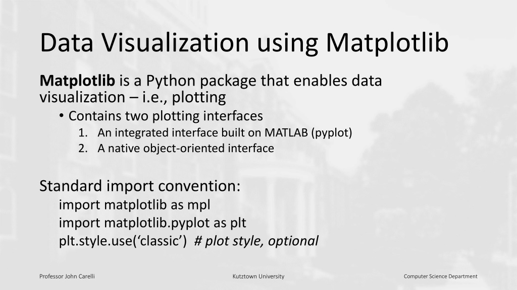


Data Visualization using Matplotlib
Matplotlib
is a Python package that enables data
visualization – i.e., plotting
•
Contains two plotting interfaces
1.
An integrated interface built on MATLAB (pyplot)
2.
A native object-oriented interface
Standard import convention:
import matplotlib as mpl
import matplotlib.pyplot as plt
plt.style.use(‘classic’)
# plot style, optional
Basic Operation
•
Get some data
x = np.linspace(0, 10, 101)
•
Plot the data
plt.plot(x
,
np.sin(x))
•
repeat to add figures to the plot
plt.plot(x, np.cos(x))
•
colors are automatically cycled
MATLAB vs. OO Interface
Matplotlib was originally written to provide a Python accessible
alternative to plotting in MATLAB
•
Designed to look familiar to MATLAB users
•
For simple plots, it can be easier to use
Object Oriented interface provides access to underlying objects
•
Provides more direct control over more complex plots
Multiple Plots, MATLAB style
# create a figure to hold the plots
plt.figure()
x = np.linspace(0, 10, 100)
# some data
# create a first panel and set the axis
plt.subplot(2, 1, 1) # (rows, columns, panel #)
plt.plot(x, np.sin(x))
# create a second panel and set the axis
plt.subplot(2, 1, 2)
plt.plot(x, np.cos(x))
•
The subplot() function creates
panels in the active figure
•
When a new subplot is created,
it becomes active
•
new plots created in that figure
Multiple Plots, OO style
# some data
x = np.linspace(0, 10, 100)
# create a grid of subplots
fig, ax = plt.subplots(2)
# fig is the figure
# ax is an array of Axes objects
# Call the plot method on each Axes object
ax[0].plot(x, np.sin(x))
ax[1].plot(x, np.cos(x))
•
The subplots() function creates
a figure and an array of axes
•
Each axis is independently
accessible
Displaying Plots
The procedure for displaying a plot varies depending on
the Python platform being used
Principal platforms:
•
A Python script
•
IPython shell
•
Either interactively or in a (Jupyter) notebook
Script Display
•
Place the plotting code in a
Python script
•
Add the show() function to
display the plot
•
Program will suspend until
the displayed plot is closed
IPython Display
%matplotlib
magic function
•
use plt.figure() to create a
canvas to draw on
•
can use plt.draw() to plot
updates
execute statements interactively
Notebook Display
%matplotlib
magic function
•
two options:
notebook
(default)
and
inline
•
in either case, show() is not needed
– plot is displayed immediately
%matplotlib notebook
•
plot is interactive (can zoom, scroll,
etc.)
%matplotlib inline
•
pdf of plot is displayed (not
interactive)
execute statements in cells
Customizing Plots
Plot appearance can be modified in a variety of ways
•
Plot style - See styles
here
•
Line colors
•
Line styles
•
Axes limits
•
Labels
Line Color
Line color can be controlled with the color parameter
•
By default, plots cycle through a pre-determined set of colors
Color Option Examples
plt.plot(x, y, color='blue') # name
plt.plot(x, y, color='g') # color code
plt.plot(x, y, color='0.75') # grayscale
plt.plot(x, y, color='#FF0000') # hex
plt.plot(x, y, color=(1.0, 0.0, 0.0)) # RBG
plt.plot(x, y, color='papayawhip') # HTML
Line Style
Controlled with the linestyle parameter
•
by name or with a character code
Axis Limits
•
Set each axis individually
plt.xlim(xmin, xmax)
plt.ylim(ymin, ymax)
•
Set them all at once
plt.axis([xmin, xmax, ymin, ymax])
•
Automatically compute the limits
plt.axis('tight’)•
Make axis units equal
plt.axis('equal')Basic Labeling
•
Plot Title
plt.title("My Awesome Plot")•
Axis Labels
plt.xlabel("x")plt.ylabel("y")•
Plot Legend
plt.legend()
Method name discrepancies
•
Most plt functions translate directly to ax methods
•
But some to be aware of:
plt.xlabel() → ax.set_xlabel()
plt.ylabel() → ax.set_ylabel()
plt.xlim() → ax.set_xlim()
plt.ylim() → ax.set_ylim()
plt.title() → ax.set_title()
•
ax.set() can be used to set multiple properties at once
Markers and Scatter Plots
•
Data point markers can be added
plt.plot(x, y, 'o', color='black’)
•
Some common markers
‘o’ ‘.’ ‘,’ ‘x’ ‘+’ ‘v ‘^’ ‘<‘ ‘>’ ‘s’ ‘d’
•
scatter method for specialized scatter plots
plt.scatter(x, y, marker=‘+’)
•
many additional options for controlling marker size,
transparency (alpha), colors, etc.
Histograms
•
Create using the hist() method
data = np.random.randn(1000)
plt.hist(data, bins=10)
•
bins option
•
integer specifying the number of bins to create
•
or a sequence specifying the edges of each bin
Bar Charts
•
bar() method for vertical charts
•
barh() for horizontal
Saving Figures to a File
•
Use the savefig() method on the figure object
# create a plot window
fig = plt.figure()
# generate the figure
fig.savefig('my_figure.png’)•
Find out what image formats are supported
fig.canvas.get_supported_filetypes()
Matplotlib is a powerful Python package for data visualization, offering both an integrated interface (pyplot) and a native object-oriented interface. This tool enables users to create various types of plots and gives control over the visualization process. Learn about basic operations, differences between MATLAB and OO interfaces, creating multiple plots in MATLAB style versus OO style, and how to display plots in different Python platforms. Explore the possibilities of Matplotlib for enhancing your data visualization skills.

Download Presentation

Please find below an Image/Link to download the presentation.
The content on the website is provided AS IS for your information and personal use only. It may not be sold, licensed, or shared on other websites without obtaining consent from the author. Download presentation by click this link. If you encounter any issues during the download, it is possible that the publisher has removed the file from their server.
E N D
Presentation Transcript
Data Visualization using Matplotlib Matplotlib is a Python package that enables data visualization i.e., plotting Contains two plotting interfaces 1. An integrated interface built on MATLAB (pyplot) 2. A native object-oriented interface Standard import convention: import matplotlib as mpl import matplotlib.pyplot as plt plt.style.use( classic ) # plot style, optional Professor John Carelli Kutztown University Computer Science Department
Basic Operation Get some data x = np.linspace(0, 10, 101) Plot the data plt.plot(x, np.sin(x)) repeat to add figures to the plot plt.plot(x, np.cos(x)) colors are automatically cycled Professor John Carelli Kutztown University Computer Science Department
MATLAB vs. OO Interface Matplotlib was originally written to provide a Python accessible alternative to plotting in MATLAB Designed to look familiar to MATLAB users For simple plots, it can be easier to use Object Oriented interface provides access to underlying objects Provides more direct control over more complex plots Professor John Carelli Kutztown University Computer Science Department
Multiple Plots, MATLAB style The subplot() function creates panels in the active figure When a new subplot is created, it becomes active new plots created in that figure # create a figure to hold the plots plt.figure() x = np.linspace(0, 10, 100) # some data # create a first panel and set the axis plt.subplot(2, 1, 1) # (rows, columns, panel #) plt.plot(x, np.sin(x)) # create a second panel and set the axis plt.subplot(2, 1, 2) plt.plot(x, np.cos(x)) Professor John Carelli Kutztown University Computer Science Department
Multiple Plots, OO style The subplots() function creates a figure and an array of axes Each axis is independently accessible # some data x = np.linspace(0, 10, 100) # create a grid of subplots fig, ax = plt.subplots(2) # fig is the figure # ax is an array of Axes objects # Call the plot method on each Axes object ax[0].plot(x, np.sin(x)) ax[1].plot(x, np.cos(x)) Professor John Carelli Kutztown University Computer Science Department
Displaying Plots The procedure for displaying a plot varies depending on the Python platform being used Principal platforms: A Python script IPython shell Either interactively or in a (Jupyter) notebook Professor John Carelli Kutztown University Computer Science Department
Script Display Place the plotting code in a Python script Add the show() function to display the plot Program will suspend until the displayed plot is closed import matplotlib.pyplot as plt import numpy as np x = np.linspace(0, 10, 100) plt.plot(x, np.sin(x)) plt.plot(x, np.cos(x)) plt.show() Professor John Carelli Kutztown University Computer Science Department
IPython Display %matplotlib import matplotlib.pyplot as plt import numpy as np %matplotlib magic function use plt.figure() to create a canvas to draw on can use plt.draw() to plot updates x = np.linspace(0, 10, 100) fig = plt.figure() plt.plot(x, np.sin(x)) plt.plot(x, np.cos(x)) execute statements interactively Professor John Carelli Kutztown University Computer Science Department
Notebook Display %matplotlib magic function two options: notebook (default) and inline in either case, show() is not needed plot is displayed immediately %matplotlib notebook plot is interactive (can zoom, scroll, etc.) %matplotlib inline pdf of plot is displayed (not interactive) %matplotlib inline import matplotlib.pyplot as plt import numpy as np x = np.linspace(0, 10, 100) plt.plot(x, np.sin(x)) plt.plot(x, np.cos(x)) execute statements in cells Professor John Carelli Kutztown University Computer Science Department
Customizing Plots Plot appearance can be modified in a variety of ways Plot style - See styles here Line colors Line styles Axes limits Labels Professor John Carelli Kutztown University Computer Science Department
Line Color Line color can be controlled with the color parameter By default, plots cycle through a pre-determined set of colors Color Option Examples plt.plot(x, y, color='blue') # name plt.plot(x, y, color='g') # color code plt.plot(x, y, color='0.75') # grayscale plt.plot(x, y, color='#FF0000') # hex plt.plot(x, y, color=(1.0, 0.0, 0.0)) # RBG plt.plot(x, y, color='papayawhip') # HTML Professor John Carelli Kutztown University Computer Science Department
Line Style Controlled with the linestyle parameter by name or with a character code plt.plot(x, y, linestyle='solid') plt.plot(x, y, linestyle='dashed') plt.plot(x, y, linestyle='dashdot') plt.plot(x, y, linestyle='dotted') plt.plot(x, y, linestyle='-') plt.plot(x, y, linestyle='--') plt.plot(x, y, linestyle='-.') plt.plot(x, y, linestyle=':') Professor John Carelli Kutztown University Computer Science Department
Axis Limits Set each axis individually plt.xlim(xmin, xmax) plt.ylim(ymin, ymax) Set them all at once plt.axis([xmin, xmax, ymin, ymax]) Automatically compute the limits plt.axis('tight ) Make axis units equal plt.axis('equal') Professor John Carelli Kutztown University Computer Science Department
Basic Labeling Plot Title plt.title("My Awesome Plot") Axis Labels plt.xlabel("x") plt.ylabel("y") Plot Legend plt.legend() Professor John Carelli Kutztown University Computer Science Department
Method name discrepancies Most plt functions translate directly to ax methods But some to be aware of: plt.xlabel() ax.set_xlabel() plt.ylabel() ax.set_ylabel() plt.xlim() ax.set_xlim() plt.ylim() ax.set_ylim() plt.title() ax.set_title() ax.set() can be used to set multiple properties at once Professor John Carelli Kutztown University Computer Science Department
Markers and Scatter Plots Data point markers can be added plt.plot(x, y, 'o', color='black ) Some common markers o . , x + v ^ < > s d scatter method for specialized scatter plots plt.scatter(x, y, marker= + ) many additional options for controlling marker size, transparency (alpha), colors, etc. Professor John Carelli Kutztown University Computer Science Department
Histograms Create using the hist() method data = np.random.randn(1000) plt.hist(data, bins=10) bins option integer specifying the number of bins to create or a sequence specifying the edges of each bin Professor John Carelli Kutztown University Computer Science Department
Bar Charts bar() method for vertical charts barh() for horizontal Professor John Carelli Kutztown University Computer Science Department
Saving Figures to a File Use the savefig() method on the figure object # create a plot window fig = plt.figure() # generate the figure fig.savefig('my_figure.png ) Find out what image formats are supported fig.canvas.get_supported_filetypes() Professor John Carelli Kutztown University Computer Science Department