Exploring Proteomics Data Analysis Workflows in Perseus
This content provides a detailed walkthrough of utilizing Perseus interface/functions for analyzing label-free and SILAC datasets in the field of proteomics. It covers loading, filtering, visualization, log transformation, rearrangement of columns, and advanced analysis techniques such as scatter plots and multiscatter plots. The content also includes instructions on filtering rows based on numerical values and comparing changes in Pearson correlation values between datasets.

Download Presentation

Please find below an Image/Link to download the presentation.
The content on the website is provided AS IS for your information and personal use only. It may not be sold, licensed, or shared on other websites without obtaining consent from the author. Download presentation by click this link. If you encounter any issues during the download, it is possible that the publisher has removed the file from their server.
E N D
Presentation Transcript
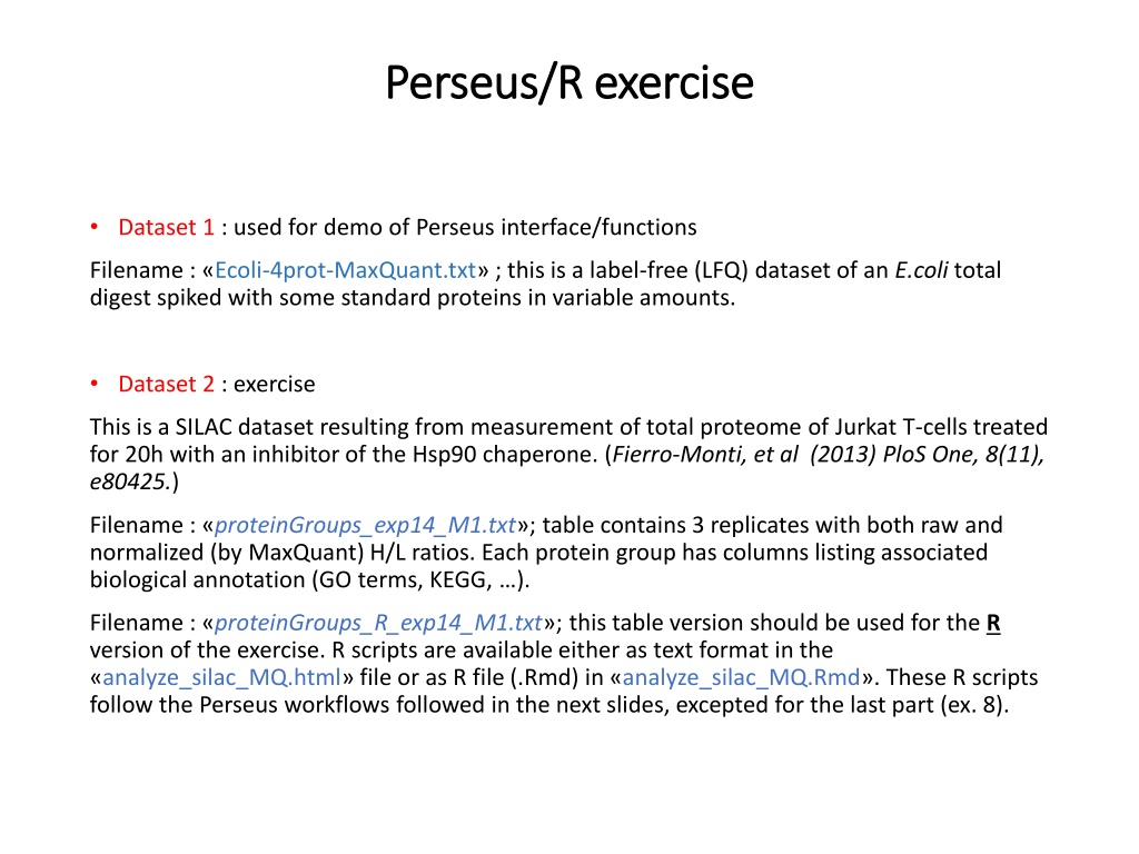
Perseus Perseus/R /R exercise exercise Dataset 1 : used for demo of Perseus interface/functions Filename : Ecoli-4prot-MaxQuant.txt ; this is a label-free (LFQ) dataset of an E.coli total digest spiked with some standard proteins in variable amounts. Dataset 2 : exercise This is a SILAC dataset resulting from measurement of total proteome of Jurkat T-cells treated for 20h with an inhibitor of the Hsp90 chaperone. (Fierro-Monti, et al (2013) PloS One, 8(11), e80425.) Filename : proteinGroups_exp14_M1.txt ; table contains 3 replicates with both raw and normalized (by MaxQuant) H/L ratios. Each protein group has columns listing associated biological annotation (GO terms, KEGG, ). Filename : proteinGroups_R_exp14_M1.txt ; this table version should be used for the R version of the exercise. R scripts are available either as text format in the analyze_silac_MQ.html file or as R file (.Rmd) in analyze_silac_MQ.Rmd . These R scripts follow the Perseus workflows followed in the next slides, excepted for the last part (ex. 8).
Perseus workflow - 1 1) LOAD MATRIX M1 Generic matrix upload (green arrow in the upper left corner); load all columns as preconfigured ; click OK. 2) FILTER Filter rows -> Filter rows based on categorical columns -> remove Reverse Filter rows -> Filter rows based on categorical columns -> remove Contaminants Filter rows -> Filter rows based on categorical columns -> remove Contaminants 2 => 4989 protein groups left. 3) ANALYSIS 1 3.1) Visualization --> histogram of all main columns (all Ratio H/L . columns) ; click on "tools" icon on the upper left of the histogram window; change max value to 4.0 => look at distributions: => H/L ratios should ideally be around 1.0 but are not => normalized ratios are at 1.0. 3.2) Basic --> summary statistics (columns) : calculate summary statistics and look at median /average of all columns. 3.3) Visualization --> scatter plot (columns): select to display "id" and "Ratio H/L exp14 rep1 20h" (or any other ratio column) note distribution of ratios ; is it easy to evaluate the data with ratios in linear form?
Perseus workflow - 2 4) LOG AND SELECT NORMALIZED COLUMNS 4.1) Basic-> transform -> log2(x) of all main columns ; click OK 4.2) Rearrange -> reorder/remove columns ; remove (send them to the left )the raw, non normalized ratio columns. Only keep the 3 normalized ratios columns ; click OK. 5) ANALYSIS 2 5.1) Visualization --> scatter plot (columns) of "id" and replicate 1; on the left select "tools" icon ; add horizontal/vertical zero lines on the left select magnifying lens tool and activate "rectangular selection" above the "points" panel on the right window, select "Gene names" in the pulldown menu control+click/drag in the plot to select points above/below the main the data cloud; change their color using the rainbow wheel on the right switch to display other replicates; check to see if the proteins selected previously are reproducibly increasing/decreasing in the treated sample (H) relative to the untreated (L). 5.2) Visualization --> multiscatter plot (default parameters ; click OK): in multiscatter plot pulldown menu select "Pearson correlation" and display values; use the Acrobat icon to save the image of the plot. 6) MORE FILTERING 6.1) Filter rows -> filter based on numerical/main column -> filter for x>2 peptides (=> 4369 protein groups left). 6.2) Re-do the multiscatter plot as before => Save plot. Compare multiscatter plots; What change do you observe in the Pearson correlation values ? ******************** proteinGroups_exp14_M2.txt contains all changes to this point.
Perseus workflow - 3 7) STATISTICAL TESTS 7.1) Tests-> One sample tests -> T-test (default parameters, includes FDR filtering); specify the suffix "FDR" in the box at the bottom; click OK 7.2) How many proteins pass T-test+FDR (column "T-test significant") (=> 339) 7.3) Repeat T-test without Benjamini-Hochberg FDR filtering: select "p-value" in the pull down box "Use for truncation" type "pval" in the "suffix" box; click OK. How many proteins pass T-test with p-value at 0.05 and without FDR and? (=> 1576) ************* proteinGroups_exp14_M3.txt contain everything up to here. 8) BIOLOGICAL ANNOTATION Do statistical test on GO and other annotations to see if any is enriched in the proteins changing in the experiment: 8.1) Annot. columns -> Fisher exact test -> select column "T-test significant FDR" ; click OK Comment on results , i.e. "Category value ************* GO-term_result_FDR.txt contains results of this step. 8.2) Find out which proteins have the enriched annotation : go back to data matrix filter rows based on categorical columns --> select annotation of interest; select Mode-> keep matching rows; select Filter Mode-> reduce matrix ; click OK; you can save the obtainedtable : Menu bar on top right Generic Matrix export ; save where desired as .txt.