Understanding the Chi-Square Test in Statistics

The Chi-square test is a fundamental statistical technique for analyzing count or frequency data. It is commonly used to determine if there is a significant difference between categorical variables like gender or disease type. The test relies on the Chi-square distribution and compares observed frequencies with expected frequencies based on a null hypothesis. This method is valuable for examining proportions in various scenarios such as the goodness-of-fit and contingency tables. By utilizing the Chi-square test appropriately, researchers can gain insights into the relationships within their data sets.

Uploaded on Sep 12, 2024 | 2 Views
Download Presentation

Please find below an Image/Link to download the presentation.
The content on the website is provided AS IS for your information and personal use only. It may not be sold, licensed, or shared on other websites without obtaining consent from the author. Download presentation by click this link. If you encounter any issues during the download, it is possible that the publisher has removed the file from their server.
E N D
Presentation Transcript
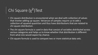
The chi-square test is the most frequently employed statistical technique for the analysis of count or frequency data. For example we may know for a sample of hospitalized patients how many are male and how many are female. For the same sample we may also know how many have complications and how many did not have complications. We may wish to know, for the population from which the sample was drawn, if the development of complications differs according to gender. The test is designated by the Greek letter chi ( ) and the distribution is called chi-square distribution which has a shape quite different from the general normal distribution of having a value between 0 and infinity. It can not take on negative values, since it is the sum of values that have been squared.
The characteristics of chi distribution; 1. It always takes a positive value 2. It may be derived from the normal distribution, so no need for the assumption that the sample is taken from normally distributed population 3. It has one accepting region and one rejecting region. 4. The degree of freedom depend on the number of groups of subgroups than on the sample size
to test the significance of difference for the qualitative data (categorical variables) such as marital status, sex, and disease type, etc.., comparing different proportion and test the significance of difference between these proportions by employing or using the frequency in the calculation to reach the conclusion. Chi-square test is most appropriate for use
number of objects or subjects in our sample that fall into the various categories of the variable of interest) and an expected frequency (the number of objects or subjects in our sample that we would expect to observe if some null hypothesis about the variable is true). We have an observed frequency (the
The chi-square test has the following formula;
Applications of Chi-square test: 1. Goodness-of-fit 2. The 2 x 2 chi-square test (contingency table, four fold table) 3. The a x b chi-square test (r x c chi-square test)
1- Goodness of fit: In this application of chi square test we are going to test the goodness of fit of sample distribution (observed frequency "O") of a qualitative variable of one sample with a theoretical (preconceived or hypothesized) distribution (theoretical, expected, estimated frequency "E"), that could be one of the following theoretical distributions; Normal population distribution, Prevalence, Incidence, or Ratio.
Example; The following data represents the sex distribution of patients with duodenal ulcer (DU). A sample of 120 patients were selected randomly from patients with DU, they were 70 males and 50 females. What is your conclusion if you know that M:F ratio in the population is 1.1:1 (use =0.05). Percentage of males with DU = 70/120 x 100 = 58.3% Percentage of females with DU = 50/120 x 100 = 41.7%
Data: Data represent a sample of DU patients selected randomly, 58.3% males and 41.7% females with 1.1:1 M:F ratio in the population. Assumption: We assume that the sample of 120 DU patients was selected randomly from a population of DU patients. HO: There is no significant difference between the proportions of males and females with DU proportions. OR There is no significant association between sex and DU. from population
HA: There is significant difference between the proportions of males and females population proportions. OR There is significant association between sex and DU. Level of significance; ( = 0.05); 5% Chance factor effect area 95% Influencing factor (association between DU and sex) d.f.=K-1; (K=Number of subgroups). with DU from effect area
Apply significance the proper test of
= 0.8015 + 0.8829 = 1.6844 (calculated value) (Calculated chi) 1.6844 < 3.841 Since Calculated < Tabulated So P>0.05 Then accept Ho.... (Ho Not rejected)
There is no significant difference between the proportions of males and females with population proportions. There is no significant association between sex and DU Sex distribution in patients with DU follows the sex distribution in the population DU from
2- 2x2 chi square test: Sometimes when we consider two groups for comparison and the variable of interest have a criteria of two in the classification, so the data here will be cross classified in a manner resulted in a contingency table consisting of two rows and two columns, such a table is referred to as 2x2 or four- fold or contingency table. For such table the degree of freedom will be determined by applying the rule of (r-1)(c-1) which will result in (2- 1)(2-1)= 1x1=1 degree of freedom. In this application of chi square test we are going to compare the of sample distribution (observed frequency "O") of a qualitative variable of two samples with a theoretical (preconceived or hypothesized) distribution (theoretical, expected, estimated frequency "E"), that can be estimated using the following rule
Total of row (Tr); Total of column (Tc); Grand total (Trc) for each cell.
Example; A researcher interested in studying the association between cancer of bladder (ca bladder) and smoking. He took the records of 20 patients with ca bladder and compared them with 200 healthy control subjects selected at random from the population. He found that half of patients with ca bladder were smokers and only 20 of the healthy controls were smoker. What is the conclusion he reached from such data (use =0.05). Percentage of smoking in ca bladder = 10/20 x 100 = 50% Percentage of smoking in healthy subjects = 20/200 x 100 = 10%
Data: Data represent two samples, the first one consist of 20 patients with ca bladder, half of them smokers (50%), and the other sample of 200 healthy subjects, 10% of them were smoker. Assumption: We assume that the two independent groups were selected randomly from two independent populations. HO: There is no significant difference between the proportions of smokers and non-smoker with or without ca bladder. OR There is no significant association between smoking and ca bladder.
HA :There is significant difference between the proportions of smokers and non- smoker with or without ca bladder. OR There is significant association between smoking and ca bladder. Level of significance; ( = 0.05); 5% chance factor effect area 95% influencing factor effect area (association between ca baldder and smoking) d.f.=(r-1)(c-1)= (2-1)(2-1)=1x1=1
Since Calculated > Tabulated So P< 0.05 Then reject Ho and accept HA There is significant difference between the proportions of smokers and non-smoker with or without ca bladder. There is significant association between smoking and ca bladder Smokers with high proportion to develop ca bladder 50% versus 10%, means five times more to develop ca bladder than healthy subjects.
3- a x b chi square test: The same application as 2x chi square test, but there are either more groups than two or the qualitative variable of interest is classified to more than two categories so we will have 2x3 or 3x2 or 3x3 etc so we have r=2 or more and c=2 or more. The difference will be seen in the degree of freedom it will be more than 1.
Important notes in chi-square test; 1- When 2x2 chi-square test have a zero cell (one of the four cells is zero) we can not apply chi-square test because we have what is called a complete dependence criteria. But for a x b chi-square test and one of the cells is zero when can not apply the test unless we do proper categorization to get rid of the zero cell. 2- When we apply 2x2 chi-square test and one of the expected cells was <5 or when we apply a x b chi-square test and one of the expected cells was <2, or when the grand total is <40 we have to apply Yates' correction formula;
3- In case of 2x2 or a x b or even goodness of fit result in significant difference in proportion and significant association, the significancy came from that cell that have a "small " value of more than 3.841
")


")


; Total of")