Development of Quantum Statistics in Quantum Mechanics

The development of quantum statistics plays a crucial role in understanding systems with a large number of identical particles. Symmetric and anti-symmetric wave functions are key concepts in quantum statistics, leading to the formulation of Bose-Einstein Statistics for bosons and Fermi-Dirac Statistics for fermions. Bose-Einstein Statistics describes the energy distribution among bosons, while Fermi-Dirac Statistics relates to fermions, each having specific spin angular momenta. These statistics govern the behavior of particles at the quantum level, providing insights into their energy distributions and quantum states.
- Quantum Statistics
- Quantum Mechanics
- Symmetric Wave Function
- Anti-symmetric Wave Function
- Bose-Einstein Statistics

Uploaded on Sep 14, 2024 | 1 Views
Download Presentation

Please find below an Image/Link to download the presentation.
The content on the website is provided AS IS for your information and personal use only. It may not be sold, licensed, or shared on other websites without obtaining consent from the author. Download presentation by click this link. If you encounter any issues during the download, it is possible that the publisher has removed the file from their server.
E N D
Presentation Transcript
M.S.P. Mandals Deogiri College,Aurangabad Department of Physics Class :- B. Sc. S. Y. (sem lll) course:-Mathematical Statistical physics and Relativity chapter:- quantum statistics Mrs. S.B.Patil
Development of Quantum Statistics For developing a quantum statistical theory for a system containing a large number of identical and indistinguishable particles, it is necessary to consider the wavefunction for many body state as (r1-- , r2-- ,r3-- ,.......) where r1-- , r2-- ,r3-- ,....are position vectors of the first, second, third ... particles respectively. Symmetric wavefunction : If on interchanging any pair of identical particles, there is no change of the sign of the wave function, i.e., if (r2-- , r1-- ,r3-- ,.......) = + (r1-- , r2-- ,r3-- ,.......) the wavefunction is said to be symmetric. .
Anti-symmetric wavefunction : If on interchanging any pair of identical particles, the sign of the wavefunction changes, i.e., if (r2-- , r1-- ,r3-- ,.......) = - (r1-- , r2-- ,r3-- ,.......) the wave function is said to be anti-symmetric. For particles having spin angular momenta that are zero or integral multiples of the unit ( h/2 ) the wave-functions are symmetric, and for particles with spin angular momenta that are odd half-integral multiples of ,the wave-functions are antisymmetric. Based on this requirement the following two quantum statistics have been developed.
Bose-Einstein Statistics This statistic was developed by S.N. Bose for light quanta, called photons and generalised by A. Einstein to describe the energy distribution among particles, whose spin angular momenta are n where n = 0, 1, 2,3,.... Such particles are called bosons. Wave functions are symmetric on interchanging two bosons. The Pauli exclusion principle which states that in each quantum state there cannot simultaneously be more than one particle, is not applicable to bosons, so that there is no upper limit to the number of bosons in a given quantum state. Examples of bosons are : particles each having spin quantum number s = 0, photon for which s=1, deutron for which s=1, mesons for which s=0
Fermi-Dirac Statistics This statistics was developed by E. Fermi for electrons and its relation to quantum mechanics was established by P.A.M. Dirac. It describes the energy distribution among particles whose spin angular momenta are (n+ ) where n = 0, 1, 2, 3, ... . In other words, they are 1 /23 /2, 5 /2....such particles are called fermions. Wave functions are antisymmetric on interchanging two fermions. The Pauli exclusion principle is applicable to fermions, so that there can be a maximum of one fermion in a given quantum state. Examples of fermions are electrons for which (s = ) , positrons for which (s = ), protons (s = ) , neutrons (s = ) ,U-mesons (s = )
Indistinguishability of Particles and its Consequences The consequences of indistinguishability of particles in quantum statistics may be explained in the following manner : Let there be two points of collection and only two cells to be occupied. In classical statistics each particle has a recognizable individuality, hence the particles are distinguishable and each particle is as likely to be 1n one cell as in the other. This means that in classical statistics, each or both of the particles can occupy any one of the two cells. Thus, in this case, we have four possible arrangements, each of which is counted for assigning a probability to the distribution. This is as shown in fig. (a)
(a) Classical p q q p pq pq Statistics (b) Bose-Einstein Statistics (c) Fermi-Dirae Statistics ** ** * * * * Fig. Essential difference in three statistics In Bose-Einstein statistics. the particles loose their individuality, hence they are indistinguishable. So We must concentrate our attention on the cell rather than the individual particles. each cell may have any number of particles. so that in this case, we have only three possible arrangements, as shown in Fig. (b).
In Fermi-Dirac statistics, since the particles are indistinguishable, again we have to concentrate our attention on the cells rather than on individual particles. But in this case, the particles obey Paul s exclusion principle according to which it is not possible to have more than one representative point in any one cell. Obviously. each cell will contain at the most one particle. Therefore, in this case, only one arrangement Is possible, as shown in Fig.(c).
Fermi- Dirac Distribution Law Consider a system consisting of n independent and indistinguishable particles. The particles pave definite energies (Or momenta) and occupy definite positions. Therefore, they can be represented by phase points in the phase space. In order to determine the energy (or momenta ) distribution of these particles in the most probable state known as equilibrium state, we divide the available volume in the phase space into large number (say k) of compartments ( quantum groups or energy levels), each compartment representing a small interval of energy (or momentum) Further each compartment is divided into elementary cells, each of size h3, where h is Planck s constants.
further We suppose that the size of the compartment is very large as compared to the size of the cell so that each compartment contains a very large number of elementary cells. let the compartment be marked 1,2,....i ....k and their mean energy values be represented by E1 , E2 ,... Ei .... Ek containing g1 , g2 ,...gi ....gk cell respectively in them. The total number of particles in the system is n= n1 + n2 + ..+ ni + nk Cur aim is to find the Fermi-Dirac distribution law i.e., the distribution of ni , Fermions out of the total n Fermions in gi cells of the i th compartment. For this, the basic postulates are.
Basic Postulates (i) The particles of indistinguishable so that there is no distinction between the various Ways in which ni , particle are chosen. (ii) The particles obey Pauli s exclusion principle according to which there can be either no particle or only one particle in a given cell. Therefore, the number of cells must be much greater than the number of particles, i.e., gi >> ni .
Out of ni number of particles in the i th compartment with mean value Ei , the first particle can be placed in any one of the available gi states, i.e., this particle can be signed to any of the g; sets of quantum numbers. Thus, the first particle can be distributed in gi different ways, in accordance with Pauli s exclusion principle and the remaining (gi +1) will remain vacant. The second particle can be arranged in (gi, +1) different ways and the process continues. Thus, the total number of different ways of arranging n, particles among available gi states with energy level , is given by - . : = gi (gi - 1) (gi- 2) (gi -3) .....[ gi - (ni - 1)] = gi !/(gi - ni ) !
Further, since the particles are indistinguishable, it would not be possible to detect any difference when n; particles are reshuffled into different ways occupied by them in the energy level Ei , Thus, out of these ni permutations of the indistinguishable particles among themselves will be meaningless. Therefore, the total number of different and distinguishable ways is = gi !/ni !(gi - ni ) ! Therefore, the thermodynamic probability for the microstate (n1 , n2 ;....ni , nk,) of the System is given by
W(n1 , n2 ;....i.k) = g1 !/n1 !(g1 n1 ) ! x g2 !/n2 !(g2 n2 ) ! x .x gi !/ni !(gi - ni ) ! .x gk !/nk !(gk - nk ) ! = gi !/ni !(gi - ni) ! ..(29) where denotes multiplication of terms for various values of i from 1 to k. -


 Classical")


 = g1 !/n1 !(g1– n1 ) ! x g2 !/n2")