Understanding Statistics: An Overview of Business Statistics in MSMSR
Learn about the core concepts of statistics in business through this MSMSR lecture plan module covering topics such as the introduction to statistics, definition of statistics, functions, scope, limitations of data, classification of data, and tabulation of data. Discover how statistics plays a crucial role in data analysis, interpretation, and decision-making in various fields. Explore real-life examples and basics of statistics like measures of central tendency and dispersion. Delve into the application of statistical models to solve complex problems and gain a better understanding of how data can be utilized effectively for decision support.

Download Presentation

Please find below an Image/Link to download the presentation.
The content on the website is provided AS IS for your information and personal use only. It may not be sold, licensed, or shared on other websites without obtaining consent from the author. Download presentation by click this link. If you encounter any issues during the download, it is possible that the publisher has removed the file from their server.
E N D
Presentation Transcript
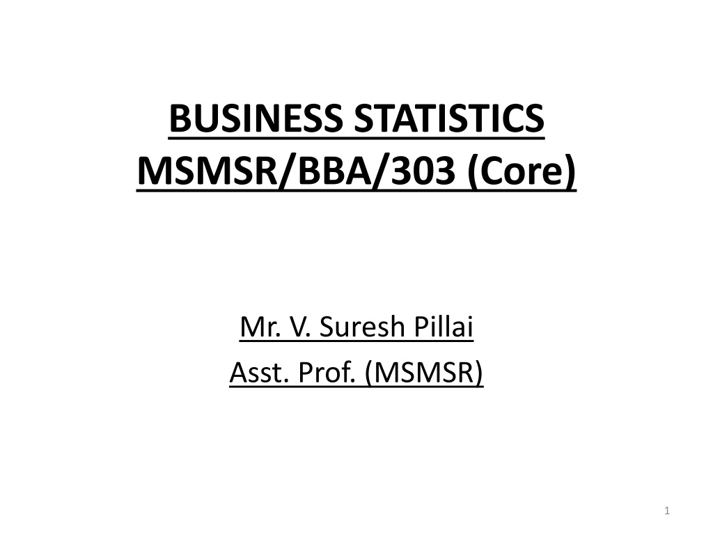
BUSINESS STATISTICS MSMSR/BBA/303 (Core) Mr. V. Suresh Pillai Asst. Prof. (MSMSR) 1
LECTURE PLAN MODULE- I S.NO. Unit Topic Proposed Date of Lecture Page No. 1. Introduction to Statistics 8th July 2022 3-4 2. Introduction Definition of Statistics 11th July 2022 5 3 Functions , Scope 12th July 2022 6-7 4 Limitations of Data. 13th July 2022 8 I 5 Classification of Data. 14th July 2022 9 6 Tabulation of Data. 15th July 2022 10 7 Tabulation of Data. 16th July2022 10 8 Practical 19th July 2022 9 Practical 20th July 2022 2
Introduction to Statistics Statistics simply means numerical data, and is field of math that generally deals with collection of data, tabulation, and interpretation of numerical data. It is actually a form of mathematical analysis that uses different quantitative models to produce a set of experimental data or studies of real life. It is an area of applied mathematics concern with data collection analysis, interpretation, and presentation. Statistics deals with how data can be used to solve complex problems. Some people consider statistics to be a distinct mathematical science rather than a branch of mathematics. Statistics makes work easy and simple and provides a clear and clean picture of work you do on a regular basis. 3
What is Statistics? Statistics is simply defined as the study and manipulation of data. As we have already discussed in the introduction that statistics deals with the analysis and computation of numerical data. Let us see more definitions of statistics given by different authors here. According to Merriam-Webster dictionary, statistics is defined as classified facts representing the conditions of a people in a state especially the facts that can be stated in numbers or any other tabular or classified arrangement . According to statistician Sir Arthur Lyon Bowley, statistics is defined as Numerical statements of facts in any department of inquiry placed in relation to each other . 4
Introduction to Statistics Statistics Examples Some of the real-life examples of statistics are: To find the mean of the marks obtained by each student in the class whose strength is 50. The average value here is the statistics of the marks obtained. Suppose you need to find how many members are employed in a city. Since the city is populated with 15 lakh people, hence we will take a survey here for 1000 people (sample). Based on that, we will create the data, which is the statistic. Basics of Statistics The basics of statistics include the measure of central tendency and the measure of dispersion. The central tendencies are mean, median and mode and dispersions comprise variance and standard deviation. Mean is the average of the observations. Median is the central value when observations are arranged in order. The mode determines the most frequent observations in a data set. Variation is the measure of spread out of the collection of data. Standard deviation is the measure of the dispersion of data from the mean. The square of standard deviation is equal to the variance. 5
Scope of Statistics Statistics is used in many sectors such as psychology, geology, sociology, weather forecasting, probability and much more. The goal of statistics is to gain understanding from the data, it focuses on applications, and hence, it is distinctively considered as a mathematical science 6
Functions or Uses of Statistics (1) Statistics helps in providing a better understanding and accurate description of nature s phenomena. (2) Statistics helps in the proper and efficient planning of a statistical inquiry in any field of study. (3) Statistics helps in collecting appropriate quantitative data. (4) Statistics helps in presenting complex data in a suitable tabular, diagrammatic and graphic form for an easy and clear comprehension of the data. (5) Statistics helps in understanding the nature and pattern of variability of a phenomenon through quantitative observations. (6) Statistics helps in drawing valid inferences, along with a measure of their reliability about the population parameters from the sample data. 7
Limitations of Data 1. Qualitative Aspect Ignored: 2. It does not deal with individual items: 3. It does not depict entire story of phenomenon: 4. It is liable to be miscued: 5. Laws are not exact: As far as two fundamental laws are concerned with statistics: 6. Results are true only on average: 7. To Many methods to study problems: 8. Statistical results are not always beyond doubt: 8
Classification of Data When data are classified with reference to geographical locations such as countries, states, cities, districts, etc., it is known as geographical classification. It is also known as spatial classification . (1) Geographical classification A classification where data are grouped according to time is known as a chronological classification. In such a classification, data are classified either in ascending or in descending order with reference to time such as years, quarters, months, weeks, etc. It is also known as temporal classification . (2) Chronological classification Under this classification, data are classified on the basis of some attributes or qualities like honesty, beauty, intelligence, literacy, marital status, etc. For example, the population can be divided on the basis of marital status (as married or unmarried) (3) Qualitative classification This type of classification is made on the basis of some measurable characteristics like height, weight, age, income, marks of students, etc (4) Quantitative classification 9
Tabulation of Data Tabulation is a systematic and logical representation of numeric data in rows and columns to facilitate comparison and statistical analysis. It facilitates comparison by bringing related information close to each other and helps in statistical analysis and interpretation. In other words, the method of placing organized data into a tabular form is known as tabulation. It may be complex, double, or simple, depending upon the nature of categorization. Objectives Of Tabulation: (1) To simplify complex data It reduces the bulk of information, i.e., it reduces raw data in a simplified and meaningful form so that it can be easily interpreted by a common man in less time. (2) To bring out essential features of data It brings out the chief/main characteristics of data. It presents facts clearly and precisely without textual explanation. (3) To facilitate comparison The representation of data in rows and columns is helpful in simultaneous detailed comparison on the basis of several parameters. (4) To facilitate statistical analysis Tables serve as the best source of organized data for statistical analysis. The task of computing average, dispersion, correlation, etc., becomes easier if data is presented in the form of a table. (5) To save space A table presents facts in a better way than the textual form. It saves space without sacrificing the quality and quantity of data. 10
LECTURE PLAN MODULE-II S.NO Module Topics Proposed Date Page no. 10 Measures of Central Tendency 21th July 2022 12 11 Introduction Types of averages 22nd July 2022 13 12 Arithmetic Mean (Simple and Weighted) 23th July 2022 14 13 Median 26th July 2022 15 14 Mode 27th July 2022 16 II 15 Graphic location of Median 28th July 2022 17 16 Mode through give Curves and Histogram 29th July 2022 18 17 Practical 30th July 2022 18 Practical 2nd Aug 2022 11
Measures of Central Tendency A measure of central tendency (also referred to as measures of centre or central location) is a summary measure that attempts to describe a whole set of data with a single value that represents the middle or centre of its distribution. There are three main measures of central tendency: the mode, the median and the mean. Each of these measures describes a different indication of the typical or central value in the distribution. 12
Introduction Types of averages The most common types of averages are the mean, median, and mode. Mean- The mean is found by adding all the numbers in a list and then divide by how many numbers there are. Let x1, x2, ... , xnbe a list. Mean = x1+ x2+...+ xnn Median The median is the middle value when a list of numbers is ordered from least to greatest or from greatest to least. Mode The mode is(are) the number(s) which occur(s) most often. Harmonic mean The harmonic mean is found by dividing the numbers of values by the sum of the reciprocals of all values. Let n be the number of values or how many numbers there are Harmonic mean=n 1xHarmonic mean=n 1x Notice that x represents a set of numbers such as {x1, x2, ... , xn} Quadratic mean The quadratic mean is found by squaring each value, adding the results, dividing by the numbers of values, and then taking the square root of that result. Quadratic mean= x2nQuadratic mean= x2nNotice again that x represents a set of numbers such as {x1, x2, ... , xn} Geometric mean Given n values that are positive, the geometric mean is the nth root of their product. Geometric mean=n x1 x2 ... xnGeometric mean=x1 x2 ... xnnWeighted mean The weighted mean is found by adding the product of each weight and each value and then dividing by the sum of all weight. Let w represents each weight and let x represent each value. Weighted mean = w x w 13
Arithmetic Mean (Simple and Weighted) Difference Simple Average Weighted Average 1. Meaning Simple average is the average of a set of values calculated with each value being assigned equal importance or weightage. Weighted average is the average of a set of values calculated by giving weightage to the relative importance of each value. 2. Formula numerator In simple average calculation, the numerator of the formula is the sum total of all the values in the set. In weighted average calculation, the numerator of the formula is the sum total of the values in the set multiplied by the weightage assigned to each value. 3. Formula denominator In simple average calculation, the denominator of the formula is the total number of values in the set. In weighted average calculation, the denominator of the formula is the sum total of all the weights assigned to the values in the set. 4. Weights assigned In simple average calculation, weights are not assigned to each value. In weighted average calculation, weights are assigned to each value in relation to their specific importance/relevance. 5. Useful when Simple average calculation is useful in simpler data analysis when all values are equally important. It is more relevant in simple mathematical analysis. Weighted average calculation finds more relevance in accounting and financial calculations such as weighted average cost of inventory, weighted average cost of capital. 6. Indication of Simple average is an indication of arithmetical mean or center point of the set of values. Weighted average on the other hand does not necessarily indicate this. It would be more tilted towards the values which have been assigned a greater weight in the set. 7. Ease of calculation Simple average is easier to calculate. Weighted average is more complex to calculate than simple average. 8. Accuracy Simple average is a less accurate method of average calculation especially in more complex sets of data. Weighted average considers the relative importance of all values and thus is a more accurate representation of the average of a set 14
Median In statistics and probability theory, the median is the value separating the higher half from the lower half of a data sample, a population, or a probability distribution. For a data set, it may be thought of as "the middle" value. The basic feature of the median in describing data compared to the mean (often simply described as the "average") is that it is not skewed by a small proportion of extremely large or small values, and therefore provides a better representation of a "typical" value. Median income, for example, may be a better way to suggest what a "typical" income is, because income distribution can be very skewed. The median is of central importance in robust statistics, as it is the most resistant statistic, having a breakdown point of 50%: so long as no more than half the data are contaminated, the median is not an arbitrarily large or small result. 15
Mode The mode is the value that appears most often in a set of data values. If X is a discrete random variable, the mode is the value x (i.e, X = x) at which the probability mass function takes its maximum value. In other words, it is the value that is most likely to be sampled. Like the statistical mean and median, the mode is a way of expressing, in a (usually) single number, important information about a random variable or a population. The numerical value of the mode is the same as that of the mean and median in a normal distribution, and it may be very different in highly skewed distributions. The mode is not necessarily unique to a given discrete distribution, since the probability mass function may take the same maximum value at several points x1, x2, etc. The most extreme case occurs in uniform distributions, where all values occur equally frequently. When the probability density function of a continuous distribution has multiple local maxima it is common to refer to all of the local maxima as modes of the distribution. Such a continuous distribution is called multimodal (as opposed to unimodal). A mode of a continuous probability distribution is often considered to be any value x at which its probability density function has a locally maximum value, so any peak is a mode. In symmetric unimodal distributions, such as the normal distribution, the mean (if defined), median and mode all coincide. For samples, if it is known that they are drawn from a symmetric unimodal distribution, the sample mean can be used as an estimate of the population mode. 16
Graphic location of Median Median and other partition values can be located on the graph of the cumulative frequency polygon (give Polygon). Suppose we have a graph of the cumulative frequency polygon as shown in the figure below: Y C U M U L A T I V E Q 3n/4 m F R E Q U I E S n/2 q n/4 o Q1 Median Q3 X Classes For median, we calculate n/2n/2. On the Y-axis we mark the height equal to n/2n/2 and from this point we draw a straight line parallel to the X-axis which intersects the polygon at point m. From point m we draw a perpendicular which touches the X-axis at M. This point on the X-axis is the median. Similarly, for the lower quartile we take a height equal to n/4n/4 on the Y-axis. From this we draw a line parallel to the X-axis which intersects the polygon at point q. From this point we draw a perpendicular on the X-axis which touches it at point Q1, which is the first quartile. For the upper quartile take the height on the Y-axis equal to 3n/43n/4 17
Mode through give Curves and Histogram A histogram consists of contiguous (adjoining) boxes. It has both a horizontal axis and a vertical axis. The horizontal axis is labeled with what the data represents (for instance, distance from your home to school). The vertical axis is labeled either frequency or relative frequency (or percent frequency or probability). The graph will have the same shape with either label. The histogram (like the stemplot) can give you the shape of the data, the center, and the spread of the data. The relative frequency is equal to the frequency for an observed value of the data divided by the total number of data values in the sample. (Remember, frequency is defined as the number of times an answer occurs.) If: f = frequency n = total number of data values (or the sum of the individual frequencies), and RF = relative frequency, then: For example, if three students in Mr. Ahab s English class of 40 students received from 90% to 100%, then, <! <newline count= 1 /> >f = 3, n = 40, and RF = = = 0.075. 7.5% of the students received 90 100%. 90 100% are quantitative measures. To construct a histogram, first decide how many bars or intervals, also called classes, represent the data. Many histograms consist of five to 15 bars or classes for clarity. The number of bars needs to be chosen. Choose a starting point for the first interval to be less than the smallest data value. A convenient starting point is a lower value carried out to one more decimal place than the value with the most decimal places. For example, if the value with the most decimal places is 6.1 and this is the smallest value, a convenient starting point is 6.05 (6.1 0.05 = 6.05). We say that 6.05 has more precision. If the value with the most decimal places is 2.23 and the lowest value is 1.5, a convenient starting point is 1.495 (1.5 0.005 = 1.495). If the value with the most decimal places is 3.234 and the lowest value is 1.0, a convenient starting point is 0.9995 (1.0 0.0005 = 0.9995). If all the data happen to be integers and the smallest value is two, then a convenient starting point is 1.5 (2 0.5 = 1.5). Also, when the starting point and other boundaries are carried to one additional decimal place, no data value will fall on a boundary. The next two examples go into detail about how to construct a histogram using continuous data and how to create a histogram using discrete data. 18
LECTURE PLAN MODULE -III S. no Module Topics Proposed date Page no. 19 III Measures of Dispersion and Skewness 3rd Aug 2022 20 20 III Part 1: Measures of Dispersion: Meaning 4th Aug 2022 21 III Calculation of Absolute and Relative measures of dispersion Range Quartile Deviation Mean Deviation Standard Deviation and Coefficient of Variation. Part 2: Measures of Skewness: Meaning of Skewness Symmetrical &Skewed Distributions Measures of Skewness Absolute and Relative Measures of Skewness Karl Pearson s Coefficient of Skewness Bowley s Coefficient of Skewness Practical Pratical 5th Aug 2022 22 23 24 25 26 27 28 29 30 31 32 33 III III III III III III III III III III III III 6th Aug 2022 10th Aug 2022 12th Aug 2022 16th Aug 2022 17th Aug 2022 18th Aug 2022 19nd Aug 2022 23rd Aug 2022 24th Aug 2022 25th Aug 2022 26th Aug 2022 27th Aug 2022 21-23 19
Measures of Dispersion and Skewness What is Dispersion? In statistics, dispersion is a measure of how distributed the data is meaning it specifies how the values within a data set differ from one another in size. It is the range to which a statistical distribution is spread around a central point. It mainly determines the variability of the items of a data set around its central point. Simply put, it measures the degree of variability around the mean value. The measures of dispersion are important to determine the spread of data around a measure of location. For example, the variance is a standard measure of dispersion which specifies how the data is distributed about the mean. Other measures of dispersion are Range and Average Deviation. What is Skewness? Skewness is a measure of asymmetry of distribution about a certain point. A distribution may be mildly asymmetric, strongly asymmetric, or symmetric. The measure of asymmetry of a distribution is computed using skewness. In case of a positive skewness, the distribution is said to be right-skewed and when the skewness is negative, the distribution is said to be left-skewed. If the skewness is zero, the distribution is symmetric. Skewness is measured on the basis of Mean, Median, and Mode. The value of skewness can be positive, negative, or undefined depending on whether the data points are skewed to left, or skewed to the right. 20
Standard Deviation and Coefficient of Variation. The standard deviation of a dataset is a way to measure how far the average value lies from the mean. To find the standard deviation of a given sample, we can use the following formula: s = ( (xi x)2/ (n-1)) where: : A symbol that means sum xi: The value of the ithobservation in the sample x: The mean of the sample n: The sample size The higher the value for the standard deviation, the more spread out the values are in a sample. However, it s hard to say if a given value for a standard deviation is high or low because it depends on the type of data we re working with. For example, a standard deviation of 500 may be considered low if we re talking about annual income of residents in a certain city. Conversely, a standard deviation of 50 may be considered high if we re talking about exam scores of students on a certain test. On way to understand whether or not a certain value for the standard deviation is high or low is to find the coefficient of variation, which is calculated as: CV = s / x where: s: The sample standard deviation x: The sample mean In simple terms, the coefficient of variation is the ratio between the standard deviation and the mean. The higher the coefficient of variation, the higher the standard deviation of a sample relative to the mean. Example: Calculating the Standard Deviation & Coefficient of Variation Suppose we have the following dataset: 21
Standard Deviation and Coefficient of Variation. Dataset: 1, 4, 8, 11, 13, 17, 19, 19, 20, 23, 24, 24, 25, 28, 29, 31, 32 Using a calculator, we can find the following metrics for this dataset: Sample mean (x): 19.29 Sample standard deviation (s): 9.25 We can then use these values to calculate the coefficient of variation: CV = s / x CV = 9.25 / 19.29 CV = 0.48 Both the standard deviation and the coefficient of variation are useful to know for this dataset. The standard deviation tells us that the typical value in this dataset lies 9.25 units away from the mean. The coefficient of variation then tells us that the standard deviation is about half the size of the sample mean. 22
Standard Deviation and Coefficient of Variation. Standard Deviation vs. Coefficient of Variation: When to Use Each The standard deviation is most commonly used when we want to know the spread of values in a single dataset. However, the coefficient of variation is more commonly used when we want to compare the variation between two datasets. For example, in finance the coefficient of variation is used to compare the mean expected return of an investment relative to the expected standard deviation of the investment. For example, suppose an investor is considering investing in the following two mutual funds: Mutual Fund A: mean = 9%, standard deviation = 12.4% Mutual Fund B: mean = 5%, standard deviation = 8.2% The investor can calculate the coefficient of variation for each fund: CV for Mutual Fund A = 12.4% / 9% = 1.38 CV for Mutual Fund B = 8.2% / 5% = 1.64 Since Mutual Fund A has a lower coefficient of variation, it offers a better mean return relative to the standard deviation. Summary Both the standard deviation and the coefficient of variation measure the spread of values in a dataset. The standard deviation measures how far the average value lies from the mean. The coefficient of variation measures the ratio of the standard deviation to the mean. The standard deviation is used more often when we want to measure the spread of values in a single dataset. The coefficient of variation is used more often when we want to compare the variation between two different datasets. 23
LECTURE PLAN MODULE- IV S. no Module Topics Proposed Date Page no. 34 IV Correlation and Regression Analysis 30th Aug 2022 25 35 IV Correlation Meaning & Definition - Uses Types Probable error 31st Aug 2022 26-28 36 IV 2nd Sept. 2022 Karl Pearson s & Spearman s Rank Correlation 37 IV Regression Meaning and Definition, Regression Equations - Problems 5th Sept. 2022 25 38 IV Practical 6th Sept. 2022 39 IV Practical 7th Sept 2022 40 IV Practical 8th Sept. 2022 41 IV Practical 9th Sept. 2022 42 IV Practical 10th Sept. 2022 43 IV Practical 13th Sept. 2022 24
Correlation and Regression Analysis The most commonly used techniques for investigating the relationship between two quantitative variables are correlation and linear regression. Correlation quantifies the strength of the linear relationship between a pair of variables, whereas regression expresses the relationship in the form of an equation. For example, in patients attending an accident and emergency unit (A&E), we could use correlation and regression to determine whether there is a relationship between age and urea level, and whether the level of urea can be predicted for a given age. Regression- In the A&E example we are interested in the effect of age (the predictor or x variable) on ln urea (the response or y variable). We want to estimate the underlying linear relationship so that we can predict ln urea (and hence urea) for a given age. Regression can be used to find the equation of this line. This line is usually referred to as the regression line. 25
Uses of correlation It is used in deriving precisely the degree, and direction of relationship between variables like price and demand, advertising expenditure and sales, rainfalls and crops yield etc 26
Probable error Probable error refers to the distance from the mean that bounds 50% of the probability mass. For asymmetric distributions, the distance on one side of the mean is generally not equal to the distance on the other side, but each distance bounds 25% of the probability mass bounded on the other side by the mean. For a Gaussian distribution, which is symmetric, the distance from the mean is about 0.6745 sigma. Classical probability theory is essential to measurement theory in the physical sciences. Random variables are used to represent unknown errors which are implicit in all nontrivial measurements. Hence the association between random variables and errors. The ordinary correlation coefficient is a function defined in a specific way on the sample space of a random variable, hence it is what is called a statistic . A common goal of sample statistics is to estimate the properties of the population from which the sample was drawn. For example, the sample mean is used as an estimator of the population mean; random fluctuations occurring in the process of drawing the sample from the population cause uncertainties in the accuracy of estimators computed from the sample. 27
Types of correlation High and Low Correlation- High correlation describes a stronger correlation between two variables, wherein a change in the first has a close association with a change in the second. Low correlation describes a weaker correlation, meaning that the two variables are probably not related. Positive, Negative, and No Correlation- A correlation in statistics denotes a linear relationship. A positive correlationmeans that this linear relationship is positive, and the two variables increase or decrease in the same direction. A negative correlationis just the opposite, wherein the relationship line has a negative slope and the variables change in opposite directions (i.e, one variable decreases while the other increases). No correlation simply means that the variables behave very differently and thus, have no linear relationship. Positive, Negative, and No Correlation: Graphical Representations. When r is greater than zero, the correlation is positive. When r is less than zero, the correlation is negative. When r = 0, there is no correlation. As the corresponding graphs show, we can conclude the following correlations: temperature and ice cream sales: the hotter the day, the higher the ice cream sales. This is a positive correlation. length of workout and body mass index (BMI): the longer the workout, the lower the BMI. This is a negative correlation. shoe size and hair color: show size has no relation to hair color. This has no correlation. Correlation Coefficient The correlation coefficient is an important statistical indicator of a correlation and how the two variables are indeed correlated (or not). This is a value denoted by the letter r, and it ranges between -1 and +1. r < 0 implies negative correlation r > 0 implies positive correlation r = 0 implies no correlation For example, if the hot days and ice cream sales correlation coefficient was found to be 0.8, this means that the correlation between the two variables is positive and strong. 28
LECTURE PLAN MODULE-IV S.no. Module Topics Proposed date Page no. 44 V Index Numbers and Probability 14th Sept. 2022 30 45 V Index Numbers-Meaning & Definition Uses Classification Construction of Index Numbers Methods of constructing 15th Sept. 2022 31-32 46 V Index Numbers Simple Aggregate Method Simple Average of Price Relative Method Weighted Index numbers 16th Sept. 2022 47 V 19th Sept. 2022 Fisher s Ideal Index (including Time and Factor Reversal tests) 48 V Consumer Price Index Problems 20th Sept. 2022 49 V Probability Theory Basic concepts of probability 21th Sept. 2022 33-36 50 V Multiplication and addition theorem of probability; conditional probability. 22nd Sept. 2022 51 V Practical 23rd Sept. 2022 52 V Practical 26th Sept. 2022 53 V Practical 27th Sept. 2022 29
Index Number An index number is a method of evaluating variations in a variable or group of variables in regards to geographical location, time, and other features. The base value of the index number is usually 100, which indicates price, date, level of production, and more. There are various kinds of index numbers. However, at present, the most relatable is the price index number that particularly indicates the changes in the overall price level (or in the value of money) for a particular time. Here, the value of money is not constant, even if it falls or rises it will affect and change the price level. An increase in the price level determines a decline in the value of money. A decrease in the price level means an increase in the value of money. Therefore, the differences in the value of money are indicated by the differences in the overall price level for a particular time. Therefore, the changes in the overall prices can be evaluated by a statistical device known as index number. Types of Index Numbers Price index number: It evaluates the relative differences in costs between two particular points in time. Quantity index number: It measures the differences in the physical quantity of the product s manufacturing, buying, or selling of one item or a group of items. 30
Definition of index numbers According to Croxton and Cowden, index numbers are devices for measuring differences in the magnitude of a group of related variables. According to Spiegal, an index number is a statistical measure designed to show changes in a variable or a group of related variables with respect to time, geographical locations, or other characteristics 31
B) Following are the important characteristics of index numbers (1) Expressed in percentage A change in terms of the absolute values may not be comparable. Index numbers are expressed in percentage, so they remove this barrier. Although, we do not use the percentage sign. It is possible to compare the agricultural production and industrial production and at the same time being expressed in percentage, we can also compare the change in prices of different commodities. (2) Relative measures or measures of net changes Index numbers measure a net or relative change in a variable or a group of variables. For example, if the price of a certain commodity rises from 10 in the year 2007 to 15 in the year 2017, the price index number will be 150 showing that there is a 50% increase in the prices over this period. (3) Measure change over a period of time or in two or more places Index numbers measure the net change among the related variables over a period of time or at two or more places. For example, change in prices, production, and more, over the two periods or at two places. (4) Specialized average Simple averages like, mean, median, mode, and more can be used to compare the variables having similar units. Index numbers are specialized average, expressed in percentage, and help in measuring and comparing the change in those variables that are expressed in different units. For example, we can compare the change in the production of industrial goods and agricultural goods. (5) Measuring changes that are not directly measurable Cost of living, business activity, and more are complex things that are not directly measurable. With the help of index numbers, it is possible to study the relative changes in such phenomena. 32
Probability theory It is a branch of mathematics that investigates the probabilities associated with a random phenomenon. A random phenomenon can have several outcomes. Probability theory describes the chance of occurrence of a particular outcome by using certain formal concepts. Probability theory makes use of some fundamentals such as sample space, probability distributions, random variables, etc. to find the likelihood of occurrence of an event. In this article, we will take a look at the definition, basics, formulas, examples, and applications of probability theory. What is Probability Theory? Probability theory makes the use of random variables and probability distributions to assess uncertain situations mathematically. In probability theory, the concept of probability is used to assign a numerical description to the likelihood of occurrence of an event. Probability can be defined as the number of favorable outcomes divided by the total number of possible outcomes of an event 33
Terms Probability Theory Basics- There are some basic terminologies associated with probability theory that aid in the understanding of this field of mathematics. Random Experiment- A random experiment, in probability theory, can be defined as a trial that is repeated multiple times in order to get a well-defined set of possible outcomes. Tossing a coin is an example of a random experiment. Sample Space- Sample space can be defined as the set of all possible outcomes that result from conducting a random experiment. For example, the sample space of tossing a fair coin is {heads, tails}. Event- Probability theory defines an event as a set of outcomes of an experiment that forms a subset of the sample space. The types of events are given as follows: Independent events: Events that are not affected by other events are independent events. Dependent events: Events that are affected by other events are known as dependent events. Mutually exclusive events: Events that cannot take place at the same time are mutually exclusive events. Equally likely events: Two or more events that have the same chance of occurring are known as equally likely events. Exhaustive events: An exhaustive event is one that is equal to the sample space of an experiment. 34
Terms Random Variable- In probability theory, a random variable can be defined as a variable that assumes the value of all possible outcomes of an experiment. There are two types of random variables as given below. Discrete Random Variable: Discrete random variables can take an exact countable value such as 0, 1, 2... It can be described by the cumulative distribution function and the probability mass function. Continuous Random Variable: A variable that can take on an infinite number of values is known as a continuous random variable. The cumulative distribution function and probability density function are used to define the characteristics of this variable. Probability -Probability, in probability theory, can be defined as the numerical likelihood of occurrence of an event. The probability of an event taking place will always lie between 0 and 1. This is because the number of desired outcomes can never exceed the total number of outcomes of an event. Theoretical probability and empirical probability are used in probability theory to measure the chance of an event taking place. Conditional Probability- When the likelihood of occurrence of an event needs to be determined given that another event has already taken place, it is known as conditional probability. It is denoted as P(A | B). This represents the conditional probability of event A given that event B has already occurred. 35
Terms Expectation- The expectation of a random variable, X, can be defined as the average value of the outcomes of an experiment when it is conducted multiple times. It is denoted as E[X]. It is also known as the mean of the random variable. Variance- Variance is the measure of dispersion that shows how the distribution of a random variable varies with respect to the mean. It can be defined as the average of the squared differences from the mean of the random variable. Variance can be denoted as Var[X]. Probability Theory Distribution Function- Probability distribution or cumulative distribution function is a function that models all the possible values of an experiment along with their probabilities using a random variable. Bernoulli distribution, binomial distribution, are some examples of discrete probability distributions in probability theory. Normal distribution is an example of a continuous probability distribution. Probability Mass Function- Probability mass function can be defined as the probability that a discrete random variable will be exactly equal to a specific value. Probability Density Function- Probability density function is the probability that a continuous random variable will take on a set of possible values 36
THANK YOU 37


")


 Following are the important")