Statistical Analysis in Birth Season Distribution
A statistical study examines birth season distribution among students, comparing the number of births in different seasons. Chi-Square tests are utilized to analyze the data and test for associations between categorical variables. An example uses the goodness-of-fit test to determine if student grades align with an expected distribution. Another example explores the influence of background music on wine purchases. The content provides insights on statistical methods and applications in various scenarios.

Download Presentation

Please find below an Image/Link to download the presentation.
The content on the website is provided AS IS for your information and personal use only. It may not be sold, licensed, or shared on other websites without obtaining consent from the author. Download presentation by click this link. If you encounter any issues during the download, it is possible that the publisher has removed the file from their server.
E N D
Presentation Transcript
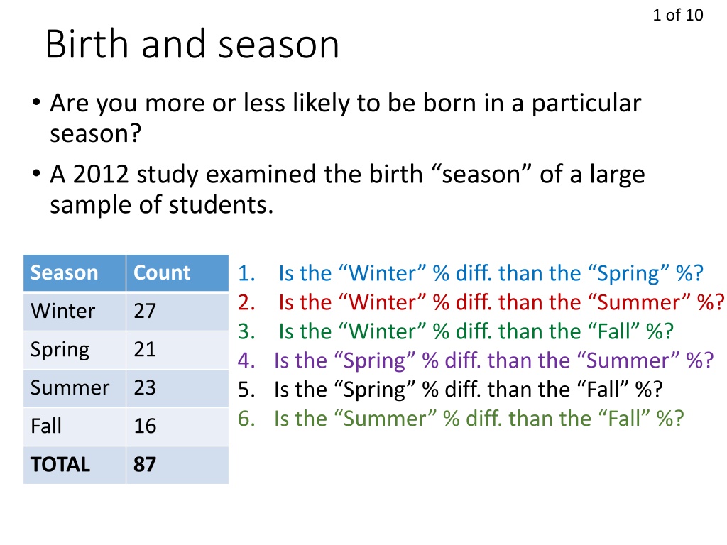
1 of 10 Birth and season Are you more or less likely to be born in a particular season? A 2012 study examined the birth season of a large sample of students. Season Count 1. 2. 3. 4. Is the Spring % diff. than the Summer %? 5. Is the Spring % diff. than the Fall %? 6. Is the Summer % diff. than the Fall %? Is the Winter % diff. than the Spring %? Is the Winter % diff. than the Summer %? Is the Winter % diff. than the Fall %? Winter 27 Spring 21 Summer 23 Fall 16 TOTAL 87
2 of 10 Chi-Square (X2) tests Use with categorical data, when proportion z-test is impractical Goodness-of-Fit (GOF) test One row or column. Is there a difference between observed (sampled) data and expected (population) data? Test of Association/Independence Matrix. Is there an association between these two categorical variables? ected E 2 2 ( exp ) O ( ) observed ected E = = 2 exp Degrees of freedom is (rows - 1)(columns 1) Conditions: Independent random samples. Individual expected values are greater than zero. E > 0 (see denominator) No more than 20% of expected values are less than 5.
3 of 10 Expected values Observed Expected E 2 O ( ) E = 2 Season Count Season Count Winter 27 Winter 21.75 Spring 21 Spring 21.75 Summer 23 Summer 21.75 = ) 1 = . . 4 ( 1 )( 1 3 d f Fall 16 Fall 21.75 . 0 25 P TOTAL 87 TOTAL 87 2 2 2 2 ( 27 21 75 . ) ( 21 21 75 . ) ( 23 21 75 . ) 16 ( 21 75 . ) = + + + = 2 . 2 885 21 75 . 21 75 . 21 75 . 21 75 .
4 of 10 EXAMPLE, X2 goodness-of-fit test Suppose that grades are expected to be roughly Normal, with most students (68%) getting C s, a few students getting B s (13.5%) and D s (13.5%), and a rare few getting A s (2.35%) and F s (2.35%). Do the grades of my Statistics students follow this distribution? Observed (O) A B C D F Total Expected (E) 86*.0235 86*.135 86*.68 86*.135 86*.0235 11 43 29 3 0 86 A B C D F 2.021 11.61 58.48 11.61 2.021 H0: HA: My Stats students follow the given distribution. My Stats students do NOT follow the given distribution. =0.05. Chi-square goodness-of-fit test. Randomness and independence are NOT met. All expected counts are greater than 0. No more than 20% are less than 5.
5 of 10 EXAMPLE, X2 goodness-of-fit test Observed (O) A B C D F Total Expected (E) 86*.0235 86*.135 86*.68 86*.135 86*.0235 11 43 29 3 0 86 A B C D F 2.021 11.61 58.48 11.61 2.021 2 2 11 ( . 2 021 ) 0 ( . 2 021 ) = + + = 2 ...... 148 03 . . 2 021 . 2 021 = ) 1 = . . 5 ( 4 d f 0005 . 0 P I reject the null hypothesis at =0.05, because P<0.05. There is significant evidence that my Stats students grades are not Normally distributed.
6 of 10 Music and Wine (matrix example) Most marker researchers believe that background music can influence the mood and purchasing behavior of customers. A study of a supermarket in Northern Ireland compares three treatments: no music, French accordion music, and Italian string music. Researchers recorded the number of bottles of French, Italian, and other wine purchased. Observed Music Wine None French Italian French 30 39 30 Italian 11 1 19 Other 43 35 35
7 of 10 Obser. Music Wine None French Italian TOTAL French 30 39 30 99 ( total . )( total . ) row column Italian 11 1 19 31 = E total . total Other 43 35 35 113 TOTAL 84 75 84 243 Expec. Music Wine None French Italian TOTAL French 34.22 30.56 34.22 99 Italian 10.72 9.57 10.72 31 Other 39.06 34.88 39.06 113 TOTAL 84 75 84 243
8 of 10 Chi-square example: Music and Wine Most marker researchers believe that background music can influence the mood and purchasing behavior of customers. A study of a supermarket in Northern Ireland compares three treatments: no music, French accordion music, and Italian string music. Researchers recorded the number of bottles of French, Italian, and other wine purchased. Expec. Music Observed Music Wine None French Italian TOTAL Wine None French Italian French 34.22 30.56 34.22 99 French 30 39 30 Italian 10.72 9.57 10.72 31 Italian 11 1 19 Other 39.06 34.88 39.06 113 Other 43 35 35 TOTAL 84 75 84 243
9 of 10 Music and Wine Most marker researchers believe that background music can influence the mood and purchasing behavior of customers. A study of a supermarket in Northern Ireland compares three treatments: no music, French accordion music, and Italian string music. Researchers recorded the number of bottles of French, Italian, and other wine purchased. H0: The distributions of wine selected are the same in all three populations of music types. The proportions of wine selected are not all the same. HA: =0.05. Chi-square test of independence/association. We will treat the subjects as SRSs from their populations. All expected counts are greater than 0. No more than 20% are less than 5.
10 of 10 Obser. Music Expec. Music Wine None French Italian TOTAL Wine None French Italian TOTAL French 34.22 30.56 34.22 99 French 30 39 30 99 Italian 10.72 9.57 10.72 31 Italian 11 1 19 31 Other 39.06 34.88 39.06 113 Other 43 35 35 113 TOTAL 84 75 84 243 TOTAL 84 75 84 243 E 2 2 2 ( ) 30 ( 34 22 . ) 35 ( 39 06 . ) O E = = + + = 2 ...... 18 279 . 34 22 . 39 06 . = ) 1 = . . 3 ( 1 )( 3 4 d f P 0025 . 0 . 0 001 I reject the null hypothesis at =0.05, because P<0.05. There is significant evidence that the type of music being played has an effect on wine sales.