Visualizing Choropleth Maps in R with tmap using CSO ESRI Shapefiles and StatBank Data

Slide Note

Learn how to create thematic choropleth maps in R using the tmap package. This tutorial covers importing ESRI shapefiles from CSO, loading StatBank data, plotting map data, and customizing map appearance with color palettes. Follow step-by-step instructions with visuals for effective spatial data visualization.

khey207 Follow

Uploaded on Sep 29, 2024 | 0 Views

Download Presentation

Please find below an Image/Link to download the presentation.

The content on the website is provided AS IS for your information and personal use only. It may not be sold, licensed, or shared on other websites without obtaining consent from the author. Download presentation by click this link. If you encounter any issues during the download, it is possible that the publisher has removed the file from their server.

E N D

Presentation Transcript

Plotting choropleth maps in R with tmap Using CSO ESRI shapefiles and StatBank data Eoin Horgan

Table of Contents 1. Introduction 2. Mapping in R 3. Importing and mapping StatBank data 2

Section 1: Introduction

Choropleth maps A choropleth map is a thematic map in which areas are shaded in proportion to the measurement of a variable. We ll cover how to make them using the tmap package in R. 4

Section 2: Mapping in R

ESRI shapefiles Install the sf package (only necessary first time using the package) install.packages("sf") Now we need to load the package before we can use it in this session (necessary once for every R session) library(sf) See http://rpubs.com/eoin-horgan-cso/tmap_code_snippets for copy/pasteable code 6

ESRI shapefiles Covers entire country in varying granularity Census 2011 files: http://census.cso.ie/censusasp/saps/boundaries/ED_SA%2 0Disclaimer1.htm Load data into variable shp: shp <- st_read("shapefile.shp", stringsAsFactors = F) Note: file is in zip archive, can use tempdir() for unzipping 7

ESRI shapefiles Examine the shapefile: > shp[, 5:7] ... NUTS3 NUTS3NAME GEOGID geometry 1 IE024 South-East (IE) R6 MULTIPOLYGON (((226795.5 90... 2 IE025 South-West (IE) R7 MULTIPOLYGON (((18146.05 95... 3 IE011 Border R1 MULTIPOLYGON (((306570.4 30... 4 IE012 Midland R5 MULTIPOLYGON (((223420.6 29... 5 IE013 West R8 MULTIPOLYGON (((48596.74 26... 8

Plotting map data Load and use the tmap package: # install.packages("tmap") library(tmap) t <- tm_shape(shp) + tm_fill(col="TOTAL2011") t This plots the total population 2011 column from the shapefile 9

Customising map appearance Colour palette: t <- tm_shape(shp) + tm_fill(col="TOTAL2011", palette = viridisLite::viridis(20), colorNA = "grey50", legend.reverse = TRUE, title = "Population 2011") t See library(tmaptools); palette_explorer() for all colour palettes http://sape.inf.usi.ch/sites/default/files/ggplot2-colour-names.png for R colours 10

Customising map appearance Fill method: t <- tm_shape(shp) + tm_fill(col="TOTAL2011", style="fisher", n = 3) t Discrete options: "cat", "fixed", "sd", "equal", "pretty", "quantile", "kmeans", "hclust", "bclust", "fisher", "jenks" and "log10_pretty" Continuous options: "cont", "order" and "log10" 11

Customising map appearance Borders t <- tm_shape(shp) + tm_fill(col="TOTAL2011") + tm_borders(col = "black", lwd = 1) t Again, colour can be any of the standard R colours 12

Customising map appearance Other options: Remove frame, increase legend size t <- tm_shape(shp) + tm_fill(col="TOTAL2011", palette = viridisLite::viridis(20), style="cont", legend.reverse = TRUE, title = "Population 2011") + tm_borders(col = "black") + tm_layout(frame = FALSE, scale = 1.6) t 13

Section 3: Importing and mapping StatBank data

Importing .px files # install.packages("pxR") library(pxR) importPX <- function(filename = "data.px"){ px <- read.px(filename) if(!is(px, "px")) stop("Input data is not a px object.") data <- as.data.frame(px) string <- names(data) remove <- c("Year", "Quarter", "Month", "value","CensusYear","HalfYear") z <- string [! string %in% remove] rowized <- dcast(data, formula=paste(paste(z, collapse= " + ")," ~ ... ")) return(rowized) } 15

Importing .px files Import table QNQ22 as the variable df Again, saving on local machine is faster df <- importPX(paste0("https://statbank.cso.ie/px/pxeirestat/", "Database/eirestat/Quarterly%20National%20Household", "%20Survey%20Main%20Results/QNQ22.px")) # or df <- importPX("C:\\Users\\path\\to\\your\\file\\QNQ22.px") 16

Data cleansing df does not match shp > levels(df$NUTS.3.Regions) "State" "Border" "Midland" "West" "Dublin" "Mid-East" "Mid-West" "South-East "South-West" Change the names so we can join correctly df$NUTS.3.Regions <- revalue(df$NUTS.3.Regions, c("South-East"="South-East (IE)", "South-West"="South-West (IE)")) The revalue function is part of the plyr package, which was imported by pxR 17

Joining data Use left_join() from dplyr for joining # install.packages("dplyr") library(dplyr) shp <- subset(shp, select = -c(NUTS1, NUTS1NAME, NUTS2, NUTS2NAME, NUTS3, MALE2011, FEMALE2011, TOTAL2011, PPOCC2011, UNOCC2011, HS2011, VACANT2011, PCVAC2011, TOTAL_AREA, LAND_AREA, CREATEDATE)) shp <- left_join(shp, df, by = c("NUTS3NAME" = "NUTS.3.Regions")) Remove unused columns, then join by region names 18

Plotting StatBank data Choose statistic and year to display var <- "2017Q2" # Choose from "1997Q4" to "2017Q2" stat <- as.character(levels(shp$Statistic)[4]) # Choose from 1 to 5 # [1] Persons aged 15 years and over in Employment (Thousand) # [2] Unemployed Persons aged 15 years and over (Thousand) # [3] Persons aged 15 years and over in Labour Force (Thousand) # [4] ILO Unemployment Rate (15 - 74 years) (%) # [5] ILO Participation Rate (15 years and over) (%) 19

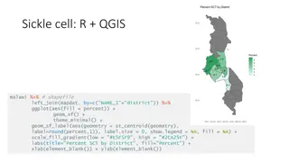
Plotting StatBank data Plot the data t <- tm_shape(shp[shp$Statistic == stat, ]) + tm_fill(col=var, palette = viridisLite::viridis(20), style = "cont", colorNA = "grey50", title = "ILO Unemployment Rate (%),\n(15 - 74 years), 2017Q2", popup.vars=c("GEOGID", var)) + tm_borders(col = "black") + tm_layout(frame = FALSE, scale = 1.1, legend.width = 0.7) t 20