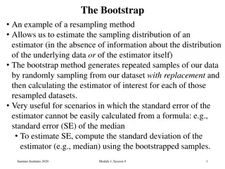
Understanding Resampling Techniques in Statistics

Explore the concept of resampling through methods like the Bootstrap, permutations, combinations, and parametric inferential statistics. Discover how resampling offers robust and relevant insights, and when to use it. Delve into the basics of permutations and combinations, and learn how to apply them creatively in statistical analysis.

Download Presentation

Please find below an Image/Link to download the presentation.
The content on the website is provided AS IS for your information and personal use only. It may not be sold, licensed, or shared on other websites without obtaining consent from the author. Download presentation by click this link. If you encounter any issues during the download, it is possible that the publisher has removed the file from their server.
E N D
Presentation Transcript
Help! Statistics! Resampling; the Bootstrap Hans Burgerhof j.g.m.burgerhof@umcg.nl May 8 2018
Help! Statistics! Lunchtime Lectures What? frequently used statistical methods and questions in a manageable timeframe for all researchers at the UMCG. No knowledge of advanced statistics is required. When? Lectures take place every 2ndTuesday of the month, 12.00-13.00 hrs. Who? Unit for Medical Statistics and Decision Making. When? Where? What? Who? Resampling: the bootstrap H. Burgerhof May 8 2018 June 12 2018 Sept 11 2018 Oct 9 2018 Room 16 Room 16 Room 16 Rode Zaal Missing data S. la Bastide Slides can be downloaded from http://www.rug.nl/research/epidemiology/download-area 2
Outline What is resampling? Definitions of permutations and combinations Some early examples of resampling Permutation test The Jackknife The basic idea of the bootstrap Some examples of bootstrapping Nonparametric bootstrap Parametric bootstrap Some more history
Resampling technicques. What and why? What is resampling? Statistical methods using permutations or subsets of the observed data (sampling within your sample) Why do we use these methods? robust, simple idea, easy to perform (with a fast computer), giving new and relevant information Why not use these methods always? - if assumptions are fulfilled, other methods are better (more efficient, more power) - for some questions, resampling cannot be used
(Parametric) inferential statistics What if we do not know if X has a normal distribution? ? population Random sample How to use the observed data in a more creative way?
Back to basics Basic terminology: what exactly are permutations and combinations? Example, we have 4 letters (A, B, C and D). How many different words of 4 letters can you make with these letters? (use each letter once) ABCD, ACDB, BCAD, BDAC, 4! = 4*3*2*1 = 24 (4 factorial = 24 permutations) 7! = 5040 10! = 3.628.800 Afbeeldingsresultaat voor scrabble
Combinations We have n different letters. In how many ways can you take a group of k letters (0 k n) without replacement, if the order does not matter? n = ! n k ( ! k )! n k n over k : the number of combinations of k from n 5 ! 5 5 4 A, B, C, D, E ABC, BCD, ACE, = = = Example: 10 3 ! 2 ! 3 2 1
Permutation test (randomisation test) Fisher, 1935 We would like to test the null hypothesis that the samples of two groups (sizes n1 and n2) are from the same distribution. We have no idea about the shape of this distribution; we do not assume normality Calculate the difference in means between the two samples: Add all observations together into one group. Sample, without replacement, n1 observations from the total group and consider those observations to be group 1 (and the other observations group 2) and calculate = Dobs x x 1 2 = Dr x x 1 1 2
Permutation test (continued) Repeat this for all possible combinations or, if this number is too large, take a random sample of combinations (Monte Carlo testing) The distribution of the calculated differences is used to test the null hypothesis of no difference or, if the number of combinations is too large, the distribution is estimated The one sided P-value is the proportion D- values larger than or equal to the observed difference
Example permutation test Do males and females have the same mean height? xm <- c(176, 180, 186, 190, 193, 170, 198) xf <- c(160, 178, 166, 180, 157, 172) mean(xm) [1] 184.71 mean(xf) [1] 168.83 D <- mean(xm) - mean(xf) D [1] 15.88
Simple program in R Data are pooled xt <- c(xm, xf) myperm <- function(x) { cc <- rep(0,1000) for (i in 1:1000) { x1 <- sample(x,7) m1 <- mean(x1) m2 <- (sum(x)-sum(x1))/6 cc[i] <- m1 - m2} cc } Vector containing1000 zeros Sample randomly 7 observations (without replacement) and calculate the mean Calculate the mean of the other 6 Put the difference between the means in the vector cc on place i res <- myperm(xt) hist(res)
Histogram of res 250 200 Frequency 150 D = 15.88 100 50 0 -20 -10 0 10 20 res pvalue <- sum(res>D)/1000 pvalue [1] 0.009 quantile (res, c(0.025,0.975)) 2.5% 97.5% -12.59 13.42
Permutation tests .. are part of non-parametric tests Fisher s exact toets is a permutation test Mann-Whitney test is a permutation test on the ranks of the observations
Jackknife http://www.visualisatie.net/internet.htm (Quenouille (1949), Tukey (1958)) In estimating an unknown parameter we think two aspects are of major importance: The estimator should be unbiased, meaning the mean of an infinite number of estimates should be equal to the real parameter we want to have an estimate of the variance of the estimator For some estimation problems we can make use of the Jackknife procedure
How does the Jackknife work? The estimator is calculated again n times, each calculation based on datasets of n 1 observations, according to the leave one out principle (in the first pseudo sample , the first observation is left out, in the second pseudo sample the second observation, and so on) Based on the n estimates, we can - make an estimate of the bias, and so a better estimate of the unknown parameter - estimate the variance of the estimator
Summary Jackknife The Jackknife uses n subsets of a sample of n observations The Jackknife estimator can reduce bias (Quenouille 1956) It gives a useful variance estimate for complex estimators It is not consistent if the estimator is not smooth, like the median It underestimates extreme value problems
Bootstrap (Efron 1979) Basic idea of the bootstrap: we have a sample of size n. Estimate the distribution of the statistic you are interested in (for example the mean) by repeatedly, with replacement, sample n observations from your original sample Using the distribution of the bootstrap-samples, you can make inference on the unknown population parameters Example: what is the mean Grade Point Average (GPA) of first year students in medicine in Groningen?
Non-parametrische bootstrap N = 16, Mean GPA = 7.12 For inference, use the bootstrap: Sample, with replacement, 16 observations and calculate the mean Repeat this1000 times GPA
Bootstrap results (1000) > quantile(res, c(0.025, 0.975)) 2.5% 97.5% 6.81 7.41 Based on the original 16 observations, if we assume normality: 7.12 2.13*0.157 [6.79 ; 7.45]
Second Bootstrap example H0: = 0 Pearson r = 0.37 Test? 60 Weight (kg) 55 height weight gewicht 175 184 168 179 . 193 73 79 64 81 50 Sample pairs repeatedly 45 88 130 140 150 160 170 180 Height (cm) lengte
Histogram of 1000 correlation coefficients, calculated Histogram of res using 1000 Bootstrap samples 200 quantile(res, c(0.025, 0.975)) 2.5% 97.5% 0.188 0.529 150 Frequency 100 Using Fisher s z-transformation: [0.16 ; 0.54] 50 0 0.0 0.1 0.2 0.3 0.4 0.5 0.6 res
Linear regression bootstrap (example from Carpenter and Bithell, 2000) 1 ounce 28.3 grams W = 0 + 1 BWT b1 = 0.68
Non-Parametric resampling Like in the correlation example, sample, with replacement, 14 cases from the original dataset and calculate the regression coefficient b1 Repeat this (at least) 1000 times Construct the 95% CI for 1 by taking percentiles of the distribution of b1 s
Non-Parametric resampling x = datamatrix, n = number of bootstrap samples mybootnon <- function(x,n) { m <- dim(x)[1] numb <- seq(1,m) resul <- rep(0,n) for (i in 1:n) {pick <- sample(numb,m,replace=T) fillx <- x[pick,1] filly <- x[pick,2] resreg <- lm(filly ~ fillx) resul[i] <- summary(resreg)$coefficients[2,1] } hist(resul) print(quantile(resul,c(0.025,0.975))) } Random bootstrap case number
Non-Parametric resampling (n = 10,000) 2.5% 97.5% 0.046 1.260
Parametric resampling We assume that the parametric model is correct. In this case: the birth weights are measured without error and the residuals are from a normal distribution with homogeneous variance ?2. We estimate ?1from the original data and estimate ?2. =?0+ ?1 ??+ ?? with Simulate 14 bootstrap data ?? ?? a random pick from N(0, ?2) Repeat this at least 1000 times and give 95% CI by percentiles of the distribution of ?1 ?
Parametric resampling (n = 10,000) 2.5% 97.5% 0.154 1.199 Smaller interval compared to nonparametric bootstrap
Linear regression bootstrap (modified example from Carpenter and Bithell) 1 ounce 28.3 grams o 15 71 318 W = 0 + 1 BWT b1 = -0.20
Results with extra case Nonparametric bootstrap 2.5% 97.5% -1.75 1.09 Parametric bootstrap 2.5% 97.5% -1.26 0.90
Some remarks on the bootstrap How many bootstrap samples? According to Carpenter and Bithell: 1000 should be enough, with fast computers 10,000 or even 100,000 is no problem (but will add hardly any new information in a lot of cases) Choosing the simulation model Only choose the parametric bootstrap if you are quite sure about the assumptions. The simulation process should mirror as closely as possible the process that gave rise to the observed data (Carpenter and Bithell, 2000)
To pull oneself up by ones bootstraps Pull yourself from the statistical swamp
In summary Permutation tests Can be a solution in testing hypotheses if the underlying distribution is unknown Jackknife Can be used in some cases to reduce bias and estimate variances Bootstrap Estimation of the distribution of a statistic
Literature Quenouille, M.H.: Notes on bias in estimation, Biometrika 1956 Efron, B. & Tibshirani, R.: An introduction to the bootstrap, Chapman and Hall 1993 Chernick, M.: Bootstrap Methods a guide for practitioners and researchers, Wiley 2008 Carpenter, J.: Bootstrap confidence intervals: when, which, what? A practical guide for medical statisticians. Statistics in Medicine , 2000 Hongyu Jiang ; Zhou Xiao-Hua: Bootstrap confidence intervals for medical costs with censored observations Statistics in Medicine, 2002
Next month Tuesday June 12 12 13 uur Room 16 Sacha la Bastide Missing Data


 inferential statistics")


")


")

")