Understanding Likelihood Weighting in Sampling
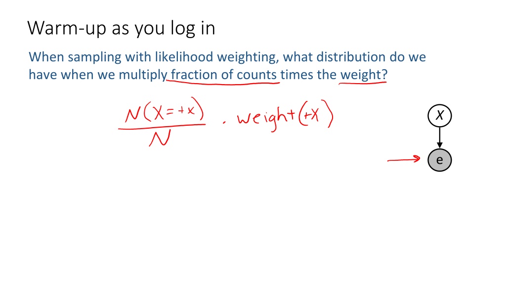
When using likelihood weighting for sampling, multiplying the fraction of counts by the weight results in a specific distribution. Likelihood weighting may fail in scenarios with high complexities, prompting the need for alternative algorithms like resampling. This technique involves eliminating unfavorable samples and generating more favorable ones to maintain a stable sample population in high-probability regions during inference processes such as robot localization.

Download Presentation

Please find below an Image/Link to download the presentation.
The content on the website is provided AS IS for your information and personal use only. It may not be sold, licensed, or shared on other websites without obtaining consent from the author. Download presentation by click this link. If you encounter any issues during the download, it is possible that the publisher has removed the file from their server.
E N D
Presentation Transcript
Warm-up as you log in When sampling with likelihood weighting, what distribution do we have when we multiply fraction of counts times the weight? X e
Announcements Assignments (everything left for the semester): HW11 (online) due Tue 4/21 P5 due Thu 4/30 HW12 (written) out Tue 4/21, due Tue 4/28 Participation points Starting now, we re capping the denominator (63 polls) in the participation points calculation Final Exam: 5/4 1-4pm (let us know by today 4/20 if you need it rescheduled) 2
Warm-up as you log in When sampling with likelihood weighting, what distribution do we have when we multiply fraction of counts times the weight? X e
AI: Representation and Problem Solving HMMs and Particle Filtering Instructors: Pat Virtue & Stephanie Rosenthal Slide credits: CMU AI and http://ai.berkeley.edu
Demo: Pacman Ghostbusters [Demos: ghostbusters (L14D1,3)]
We need a new algorithm! When |X| is more than 106 or so (e.g., 3 ghosts in a 10x20 world), exact inference becomes infeasible Likelihood weighting fails completely number of samples needed grows exponentially with T 1 LW(10) LW(100) LW(1000) LW(10000) 0.8 X0 X1 X2 X3 0.6 RMS error 0.4 E1 E2 E3 0.2 0 0 5 10 15 20 25 30 35 40 45 50 Time step
We need a new idea! t=2 t=7 The problem: sample state trajectories go off into low-probability regions, ignoring the evidence; too few reasonable samples Solution: kill the bad ones, make more of the good ones This way the population of samples stays in the high-probability region This is called resampling or survival of the fittest
Robot Localization In robot localization: We know the map, but not the robot s position Observations may be vectors of range finder readings State space and readings are typically continuous (works basically like a very fine grid) and so we cannot store B(X) Particle filtering is a main technique
Particle Filter Localization (Sonar) [Dieter Fox, et al.] [Video: global-sonar-uw-annotated.avi]
Particle Filtering Represent belief state by a set of samples Samples are called particles Time per step is linear in the number of samples But: number needed may be large 0.0 0.1 0.0 0.0 0.0 0.2 0.0 0.2 0.5 This is how robot localization works in practice
Representation: Particles Our representation of P(X) is now a list of N particles (samples) Generally, N << |X| Storing map from X to counts would defeat the point P(x) approximated by number of particles with value x So, many x may have P(x) = 0! More particles, more accuracy Usually we want a low-dimensional marginal E.g., Where is ghost 1? rather than Are ghosts 1,2,3 in {2,6], [5,6], and [8,11]? Particles: (3,3) (2,3) (3,3) (3,2) (3,3) (3,2) (1,2) (3,3) (3,3) (2,3) For now, all particles have a weight of 1
Particle Filtering: Propagate forward Particles: (3,3) (2,3) (3,3) (3,2) (3,3) (3,2) (1,2) (3,3) (3,3) (2,3) A particle in state xt is moved by sampling its next position directly from the transition model: xt+1 ~ P(Xt+1| xt) Here, most samples move clockwise, but some move in another direction or stay in place This captures the passage of time If enough samples, close to exact values before and after (consistent) Particles: (3,2) (2,3) (3,2) (3,1) (3,3) (3,2) (1,3) (2,3) (3,2) (2,2)
Particle Filtering: Observe Particles: (3,2) (2,3) (3,2) (3,1) (3,3) (3,2) (1,3) (2,3) (3,2) (2,2) Slightly trickier: Don t sample observation, fix it Similar to likelihood weighting, weight samples based on the evidence W = P(et|xt) Particles: (3,2) w=.9 (2,3) w=.2 (3,2) w=.9 (3,1) w=.4 (3,3) w=.4 (3,2) w=.9 (1,3) w=.1 (2,3) w=.2 (3,2) w=.9 (2,2) w=.4 Normalize the weights: particles that fit the data better get higher weights, others get lower weights
Particle Filtering: Resample Particles: (3,2) w=.9 (2,3) w=.2 (3,2) w=.9 (3,1) w=.4 (3,3) w=.4 (3,2) w=.9 (1,3) w=.1 (2,3) w=.2 (3,2) w=.9 (2,2) w=.4 Rather than tracking weighted samples, we resample We have an updated belief distribution based on the weighted particles (New) Particles: (3,2) (2,2) (3,2) (2,3) (3,3) (3,2) (1,3) (2,3) (3,2) (3,2) We sample N new particles from the weighted belief distributions Now the update is complete for this time step, continue with the next one
Summary: Particle Filtering Particles: track samples of states rather than an explicit distribution Propagate forward Weight Resample Particles: (3,3) (2,3) (3,3) (3,2) (3,3) (3,2) (1,2) (3,3) (3,3) (2,3) Particles: (3,2) (2,3) (3,2) (3,1) (3,3) (3,2) (1,3) (2,3) (3,2) (2,2) Particles: (3,2) w=.9 (2,3) w=.2 (3,2) w=.9 (3,1) w=.4 (3,3) w=.4 (3,2) w=.9 (1,3) w=.1 (2,3) w=.2 (3,2) w=.9 (2,2) w=.4 (New) Particles: (3,2) (2,2) (3,2) (2,3) (3,3) (3,2) (1,3) (2,3) (3,2) (3,2) Consistency: see proof in AIMA Ch. 15 [Demos: ghostbusters particle filtering (L15D3,4,5)]
Weighting and Resampling How to compute a belief distribution given weighted particles Weight Particles: (3,2) w=.9 (2,3) w=.2 (3,2) w=.9 (3,1) w=.4 (3,3) w=.4 (3,2) w=.9 (1,3) w=.1 (2,3) w=.2 (3,2) w=.9 (2,2) w=.4
Summary: Particle Filtering Particles: track samples of states rather than an explicit distribution Propagate forward Weight Resample Particles: (3,3) (2,3) (3,3) (3,2) (3,3) (3,2) (1,2) (3,3) (3,3) (2,3) Particles: (3,2) (2,3) (3,2) (3,1) (3,3) (3,2) (1,3) (2,3) (3,2) (2,2) Particles: (3,2) w=.9 (2,3) w=.2 (3,2) w=.9 (3,1) w=.4 (3,3) w=.4 (3,2) w=.9 (1,3) w=.1 (2,3) w=.2 (3,2) w=.9 (2,2) w=.4 (New) Particles: (3,2) (2,2) (3,2) (2,3) (3,3) (3,2) (1,3) (2,3) (3,2) (3,2) Consistency: see proof in AIMA Ch. 15 [Demos: ghostbusters particle filtering (L15D3,4,5)]
Piazza Poll 1 If we only have one particle which of these steps are unnecessary? Propagate forward Weight Resample Select all that are unnecessary. A. Propagate forward B. Weight C. Resample D. None of the above [Demos: ghostbusters particle filtering (L15D3,4,5)]
Piazza Poll 1 If we only have one particle which of these steps are unnecessary? Propagate forward Weight Resample Select all that are unnecessary. A. Propagate forward B. Weight C. Resample D. None of the above Unless the weight is zero, in which case, you ll want to resample from the beginning [Demos: ghostbusters particle filtering (L15D3,4,5)]
Particle Filter Localization (Laser) [Video: global-floor.gif] [Dieter Fox, et al.]
Robot Mapping SLAM: Simultaneous Localization And Mapping We do not know the map or our location State consists of position AND map! Main techniques: Kalman filtering (Gaussian HMMs) and particle methods DP-SLAM, Ron Parr [Demo: PARTICLES-SLAM-mapping1-new.avi]
Particle Filter SLAM Video 1 [Sebastian Thrun, et al.] [Demo: PARTICLES-SLAM-mapping1-new.avi]
Particle Filter SLAM Video 2 [Dirk Haehnel, et al.] [Demo: PARTICLES-SLAM-fastslam.avi]
SLAM https://www.irobot.com/


")


")