Understanding Second-Order RLC Circuits in Electronics
Explore second-order RLC circuits in electronics, characterized by second-order differential equations and involving resistors, inductors, capacitors, and voltage sources. Learn about initial and final values of voltage and current, applications in filters, and the differential equations governing these circuits.

Download Presentation

Please find below an Image/Link to download the presentation.
The content on the website is provided AS IS for your information and personal use only. It may not be sold, licensed, or shared on other websites without obtaining consent from the author. Download presentation by click this link. If you encounter any issues during the download, it is possible that the publisher has removed the file from their server.
E N D
Presentation Transcript
RLC circuits Unit-2(ECE-S202) (Atul Kr. Agnihotri ) Second-Order Circuits RLC circuits
A Bit on Second-Order Circuits A second-order circuit consists of resistors and the equivalent of two energy storage elements (Ls, Cs). A second-order circuit is characterized by a second-order differential equation (contains second-derivatives of time) Example: A circuit containing R, L and C in series with a voltage source; a circuit with R, L and C in parallel.
Initial and final values of v, i, dv/dt, and di/dt Example: The switch in this circuit has been closed for a long time. It opens at t = 0. Find: i(0+), v(0+), di(0+)/dt, dv(0+)/dt, i(infinite time), v(infinite time) a. Values for t < 0 b. Values for t = 0+ c. Values for t = infinity
A 2nd Order RLC Circuit i(t) R + vs(t) C - L Application: Filters A bandpass filter such as IF amplifier for the AM radio. A lowpass filter with a sharper cutoff than can be obtained with an RC circuit.
The Differential Equation i(t) vr(t) + - R + + vc(t) vs(t) C - - vl(t) - + KVL around the loop: L vr(t) + vc(t) + vl(t) = vs(t) 1 ( ) ( ) Ri t i x dx C ( ) 1 ( ) i t L dt LC t ( ) dt di t + + = ( ) L v t s 2 ( ) ( ) 1 L dv t dt R di t d i t dt + + = s 2
The Differential Equation The voltage and current in a second order circuit is the solution to a differential equation of the following form: 2 ( ) ( ) dt d x t dt dx t (the forcing function + + = 2 0 2 ( ) x t ( ) f t the driving voltage or 2 current source) = + ( ) x t ( ) ( ) x t x t p c xp(t) is the particular solution (forced response) and xc(t) is the complementary solution (natural response).
The Particular Solution The particular solution xp(t) is usually a weighted sum of f(t) and its first and second derivatives. If f(t) is constant, then xp(t) is constant. If f(t) is sinusoidal, then xp(t) is sinusoidal (with the same frequency as the source, for a circuit of only linear elements)
The Complementary Solution The complementary solution has the following form: ( ) = st cx t Ke K is a constant determined by initial conditions. s is a constant determined by the coefficients of the differential equation. 2 st st d Ke dt dKe dt + + = 2 0 st 2 0 Ke 2 + + = 2 2 0 st st st 2 0 s Ke sKe Ke + + = 2 2 0 2 0 s s
Characteristic Equation To find the complementary solution, we need to solve the characteristic equation: 2 0 2 s s = + + = 2 0 0 0 The characteristic equation has two roots-call them s1 and s2. ( ) K e = + s t s t c x t K e 1 2 1 2 = + 2 1 s 1 0 0 = 2 1 s 2 0 0
Overdamped, critically damped and underdamped response of source-free transiently excited 2nd-order RLC circuit Assume circuit is excited by energy stored in C or L of series RLC circuit. Assume i(t) = K1es1t + K2es2t where (with slightly different notation) s 1 + = 2 2 0 2 = 2 s where 2 0 = / 2 R L = 1 / LC = R/2L is called the damping factor and is the undamped natural frequency LC / 1 0= If > 0 overdamped case a If = critically damped case b If < underdamped case c