Applications of Time-Frequency Analysis for Filter Design

Signal decomposition and filter design techniques are explored using time-frequency analysis. Signals can be decomposed in both time and frequency domains to extract desired components or remove noise. Various transform methods like the Fourier transform and fractional Fourier transform are employed for signal processing. The concept of cutoff lines and filter design using the fractional Fourier transform are discussed in detail, showcasing the importance of analyzing signals in both time and frequency domains.

• Time-frequency analysis
• Signal decomposition
• Filter design
• Fourier transform
• Fractional Fourier transform

killian Follow

Uploaded on Aug 27, 2024 | 1 Views

Download Presentation

Please find below an Image/Link to download the presentation.

The content on the website is provided AS IS for your information and personal use only. It may not be sold, licensed, or shared on other websites without obtaining consent from the author. Download presentation by click this link. If you encounter any issues during the download, it is possible that the publisher has removed the file from their server.

Presentation Transcript

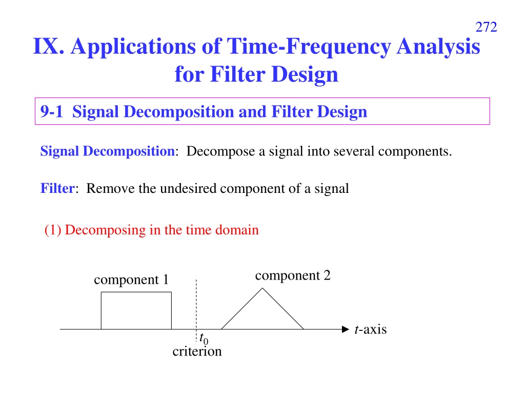
1. 272 IX. Applications of Time-Frequency Analysis for Filter Design 9-1 Signal Decomposition and Filter Design Signal Decomposition: Decompose a signal into several components. Filter: Remove the undesired component of a signal (1) Decomposing in the time domain component 2 component 1 t-axis t0 criterion

2. 273 (2) Decomposing in the frequency domain ( ) sin(4 x t t = ) cos(10 + ) t -5 -2 2 5 f-axis Sometimes, signal and noise are separable in the time domain (1) without any transform Sometimes, signal and noise are separable in the frequency domain (2) using the FT (conventional filter) = ( ) ( ( )) i ( ) x t IFT FT x t H f o If signal and noise are not separable in both the time and the frequency domains (3) Using the fractional Fourier transform and time-frequency analysis

3. 274 criterion in the time domain cutoff line perpendicular to t-axis f-axis cutoff line = t0 t-axis t-axis t0 criterion in the frequency domain cutoff line perpendicular to f-axis f-axis cutoff line f0 f-axis= f0 t-axis

4. x(t) = triangular signal + chirp noise 0.3exp[j 0.5(t 4.4)2] 275 signal + noise FT 1 1 0.5 0.5 0 0 -0.5 -0.5 -10 -5 0 5 10 -10 -5 0 5 10 reconstructed signal 3 FRFT 1 = -arccot(1/2 ) 2 0.5 1 0 0 -0.5 -10 -5 0 5 10 -10 -5 0 5 10

5. x(t) = triangular signal + chirp noise 0.3exp[j 0.5(t 4.4)2] 276 2 1.5 1 0.5 f-axis 0 -0.5 -1 -1.5 -2 -8 -6 -4 -2 0 2 4 6 t-axis 8

6. 277 Decomposing in the time-frequency distribution If x(t) = 0 for t < T1and t > T2 ( ) , 0 x W t f = for t < T1and t > T2(cutoff lines perpendicular to t-axis) If X( f ) = FT[x(t)] = 0 for f < F1and f > F2 for f < F1and f > F2(cutoff lines parallel to t-axis) What are the cutoff lines with other directions? ( ) W t f = , 0 x with the aid of the FRFT, the LCT, or the Fresnel transform

7. 278 Filter designed by the fractional Fourier transform ( ) ( ) o F F i x t O O x t ( ) = = H u ( ) ( ( )) i ( ) x t IFT FT x t H f o O means the fractional Fourier transform: F ( ) x t dt e e e 2 csc cot ( ) u 2 j j t t 2 u = cot j ( ) x t 1 cot O j F f-axis Signal noise noise noise Signal Signal FRFT FRFT t-axis cutoff line cutoff line

8. 279 ( ) ( ) ( ) = x t O O x t H u o F F i 1 0 u u u u ( ) ( ) ( ) = + If H u S u u 0 = H u 0 0 1 0 u u u u ( ) ( ) ( ) 0 = = H u S u u H u If 0 0 S(u): Step function 0 (1) cutoff line f-axis (2) u0 cutoff line ( )

9. 280 Effect of the filter designed by the fractional Fourier transform (FRFT): Placing a cutoff line in the direction of ( sin , cos ) = 0 = 0.15 = 0.35 = 0.5 (time domain) (FT)

10. 281 f-axis (0, f1) desired part cutoff line . undesired part (-t0, 0) . t-axis (t1, 0) undesired part cutoff line (0, -f0) = ? u0= ?

11. 282 The Fourier transform is suitable to filter out the noise that is a combination of sinusoid functions exp(jn1t). The fractional Fourier transform (FRFT) is suitable to filter out the noise that is a combination of higher order exponential functions exp[j(nk tk+ nk-1 tk-1+ nk-2 tk-2+ . + n2 t2+ n1 t)] For example: chirp function exp(jn2 t2) With the FRFT, many noises that cannot be removed by the FT will be filtered out successfully.

12. 283 Example (I) 4 4 10 real part imaginary part 5 2 2 0 0 0 -5 -2 -2 -10 -10 0 10 -10 0 10 -10 0 10 t axis (a) Signal s(t) (b) f(t) = s(t) + noise (c) WDF of s(t) ( ) s t ( ) = 2 2cos 5 exp( /10) t t 2 2 2 + = + + 0.23 0.3 8.5 0.46 9.6 j t j t j t j t j t ( ) 0.5 0.5 0.5 n t e e e

13. 284 10 10 10 5 5 5 0 0 0 -5 -5 -5 -10 -10 -10 -10 (d) WDF of f(t) (e) GT of s(t) (f) GT of f(t) 0 10 -10 0 10 -10 0 10 GT: Gabor transform, WDF: Wigner distribution function horizontal: t-axis, vertical: -axis

14. 285 GWT: Gabor-Wigner transform 10 10 10 5 5 5 L3 0 0 0 L1 L2 -5 -5 -5 -10 -10 -10 -10 0 10 L4 -10 (g) GWT of f(t) (h) Cutoff lines on GT 0 10 -10 (i) Cutoff lines on GWT 0 10 FrFT order

15. 286 10 10 10 5 5 5 0 0 0 -5 -5 -5 -10 -10 -10 L1 L2 -10 (j) performing the FRFT 0 10 -10 0 10 -10 (e) Cutoff lines corresponding to the high pass filter (k) High pass filter (l) GWT after filter 0 10 (d) GWT of (a) (f) GWT of (c) (performing the FRFT) and calculate the GWT 2 2 1 1 0 0 mean square error (MSE) = 0.1128% -1 -1 -2 -2 -10 0 10 -10 0 10 (h) Recovered signal (real part) and the origianl signal (g) Recovered signal (m) recovered signal (n) recovered signal (green) and the original signal (blue)

16. 287 Example (II) 3 7 . 0 exp( . 0 j 032 4 . 3 j ) t t Signal + 10 3 2 5 2 1 0 1 -5 0 0 -10 -1 -10 (a) Input signal (b) Signal + noise (c) WDF of (b) 0 10 -10 0 10 -10 0 10 10 10 2 MSE = 0.3013% 5 5 0 0 1 -5 -5 0 -10 -10 -10 (d) Gabor transform of (b) (e) GWT of (b) (f) Recovered signal 0 10 -10 0 10 -10 0 10

17. 288 [Important Theory]: Using the FT can only filter the noises that do not overlap with the signals in the frequency domain (1-D) In contrast, using the FRFT can filter the noises that do not overlap with the signals on the time-frequency plane (2-D)

18. 289 [ ] Q1: time-frequency distribution filter signal decomposition Q2: Cutoff lines

19. 290 [Ref] Z. Zalevsky and D. Mendlovic, Fractional Wiener filter, Appl. Opt., vol. 35, no. 20, pp. 3930-3936, July 1996. [Ref] M. A. Kutay, H. M. Ozaktas, O. Arikan, and L. Onural, Optimal filter in fractional Fourier domains, IEEE Trans. Signal Processing, vol. 45, no. 5, pp. 1129-1143, May 1997. [Ref] B. Barshan, M. A. Kutay, H. M. Ozaktas, Optimal filters with linear canonical transformations, Opt. Commun., vol. 135, pp. 32-36, 1997. [Ref] H. M. Ozaktas, Z. Zalevsky, and M. A. Kutay, The Fractional Fourier Transform with Applications in Optics and Signal Processing, New York, John Wiley & Sons, 2000. [Ref] S. C. Pei and J. J. Ding, Relations between Gabor transforms and fractional Fourier transforms and their applications for signal processing, IEEE Trans. Signal Processing, vol. 55, no. 10, pp. 4839-4850, Oct. 2007.

20. 291 9-2 TF analysis and Random Process For a random process x(t), we cannot find the explicit value of x(t). The value of x(t) is expressed as a probability function. Auto-covariance function Rx(t, ) ( ) , x R t E x t = In usual, we suppose that E[x(t)] = 0 for any t + ( /2) ( /2) x t E x t = + ( /2) ( /2) x t ( ) + d d ( /2, ) ( /2, ) , x t x t P 1 2 1 2 1 2 (alternative definition of the auto-covariance function: ( ) , ( ) ( x R t E x t x t = ) Power spectral density (PSD) Sx(t, f ) ( ) , x S t f ( ) = 2 j f , R t e d x

21. 292 Relation between the WDF and the random process ( ) , x E W t f E x t = ( ) ( ) = + * 2 j f / 2 / 2 x t e d ( ) 2 j f , R t e d x ( ) = 2 j f , R t e d x ( ) = , S t f x Relation between the ambiguity function and the random process ( ) ( ) , /2 x E A E x t x t ( ) ( ) = + = * 2 2 j t j t /2 , e dt R t e dt x

22. 293 Stationary random process: the statistical properties do not change with t. ( ) ( ) ( ) = = Auto-covariance function , , R t R t R 1 2 x x x for any t, ( ) E x = ( /2) ( /2) R x x ( ) = ( /2, d d ) ( /2, ) , x x P 1 2 1 2 1 2 ( ) f ( ) = 2 PSD: j f S R e d x x White noise: where is some constant. ( ) f = ( ) ( ) x R = x S

23. When x(t) is stationary, ( ) , x E W t f ( ) , x E A = 294 ( ) f = S (invariant with t) x ( ) ( ) ( ) ( ) = e = 2 2 j t j t R e dt R dt R x x x (nonzero only when = 0) a typical E[Ax( , )] for a typical E[Wx(t, f)] for g (c) W (u, ) g stationary random process (d) A ( ) stationary random process 2 2 f 0 0 -2 -2 t -2 0 2 -2 0 2

24. 295 For white noise, ( ) E W t f = , x ( ) ( ) ( ) E A = , x [Ref 1] W. Martin, Time-frequency analysis of random signals , ICASSP 82, pp. 1325-1328, 1982. [Ref 2] W. Martin and P. Flandrin, Wigner-Ville spectrum analysis of nonstationary processed , IEEE Trans. ASSP, vol. 33, no. 6, pp. 1461-1470, Dec. 1983. [Ref 3] P. Flandrin, A time-frequency formulation of optimum detection , IEEE Trans. ASSP, vol. 36, pp. 1377-1384, 1988. [Ref 4] S. C. Pei and J. J. Ding, Fractional Fourier transform, Wigner distribution, and filter design for stationary and nonstationary random processes, IEEE Trans. Signal Processing, vol. 58, no. 8, pp. 4079-4092,Aug. 2010.

25. 296 Filter Design for White noise f-axis conventional filter by TF analysis Signal t-axis white noise everywhere Esignal: energy of the signal A: area of the time frequency distribution of the signal E signal 10log SNR 10 ( , ) t f dtdf W noise ( , ) signal part t f E signal A 10log SNR The PSD of the white noise is Snoise(f) = 10

26. 297 ( ) ( ) E W t f , E A If is nonzero when 0, varies with t and , x x then x(t) is a non-stationary random process. ( ) ( ) ( ) ( ) ( ) If = + + + + h t x t x t x t x t 1 2 3 k xn(t) s have zero mean for all t s xn(t) s are mutually independent for all t s and s E x t E x t + = + = ( /2) ( /2) ( /2) ( /2) 0 x t E x t m n m n if m n, then k k = ( ) ( ) ( ) ( ) E W E W t f = , , , t f , [ , ] E A E A h x h x n n = 1 n = 1 n

27. 298 (1) Random process for the STFT E[x(t)] 0 should be satisfied. Otherwise, t B + t B + ( ) ( ) t B t B = ( ) = 2 2 j f j f [ ( , )] E X t f [ ] [ ( )] E x E x w t e d w t e d for zero-mean random process, E[X(t, f )] = 0 (2)Decompose by the AF and the FRFT Any non-stationary random process can be expressed as a summation of the fractional Fourier transform (or chirp multiplication) of stationary random process.

28. 299 -axis -axis An ambiguity function plane can be viewed as a combination of infinite number of radial lines. Each radial line can be viewed as the fractional Fourier transform of a stationary random process.

29. 300 ( ) S f white noise = ( ) S f = f ( ) S f = f ( ) S f = f 0 color noise

30. 301 Time-Frequency Analysis AD 1785 The Laplace transform was invented AD 1812 The Fourier transform was invented AD 1822 The work of the Fourier transform was published AD 1898 Schuster proposed the periodogram. AD 1910 The Haar Transform was proposed AD 1927 Heisenberg discovered the uncertainty principle AD 1929 The fractional Fourier transform was invented by Wiener AD 1932 The Wigner distribution function was proposed AD 1946 The short-time Fourier transform and the Gabor transform was proposed. In the same year, the computer was invented transform / distribution

31. 302 AD 1961 Slepian and Pollak found the prolate spheroidal wave function AD 1965 The Cooley-Tukey algorithm (FFT) was developed AD 1966 Cohen s class distribution was invented AD 1970s VLSI was developed AD 1971 Moshinsky and Quesne proposed the linear canonical transform AD 1980 The fractional Fourier transform was re-invented by Namias AD 1981 Morlet proposed the wavelet transform AD 1982 The relations between the random process and the Wigner distribution function was found by Martin and Flandrin AD 1988 Mallat and Meyer proposed the multiresolution structure of the wavelet transform; In the same year, Daubechies proposed the compact support orthogonal wavelet transform / distribution

32. 303 AD 1989 The Choi-Williams distribution was proposed; In the same year, Mallat proposed the fast wavelet transform AD 1990 The cone-Shape distribution was proposed by Zhao, Atlas, and Marks AD 1990s The discrete wavelet transform was widely used in image processing AD 1992 The generalized wavelet transform was proposed by Wilson et. al. AD 1993 Mallat and Zhang proposed the matching pursuit; In the same year, the rotation relation between the WDF and the fractional Fourier transform was found by Lohmann AD 1994 The applications of the fractional Fourier transform in signal processing were found by Almeida, Ozaktas, Wolf, Lohmann, and Pei; Boashash and O Shea developed polynomial Wigner-Ville distributions AD 1995 Auger and Flandrin proposed time-frequency reassignment L. J. Stankovic, S. Stankovic, and Fakultet proposed the pseudo Wigner distribution

33. 304 AD 1996 Stockwell, Mansinha, and Lowe proposed the S transform Daubechies and Maes proposed the synchrosqueezing transform AD 1998 N. E. Huang proposed the Hilbert-Huang transform Chen, Donoho, and Saunders proposed the basis pursuit AD 1999 Bultan proposed the four-parameter atom (i.e., the chirplet) AD 2000 The standard of JPEG 2000 was published by ISO Another wavelet-based compression algorithm, SPIHT, was proposed by Kim, Xiong, and Pearlman The curvelet was developed by Donoho and Candes AD 2000s The applications of the Hilbert Huang transform in signal processing, climate analysis, geology, economics, and speech were developed AD 2002 The bandlet was developed by Mallet and Peyre; Stankovic proposed the time frequency distribution with complex arguments

34. 305 AD 2003 Pinnegar and Mansinha proposed the general form of the S transform Liebling et al. proposed the Fresnelet. AD 2005 The contourlet was developed by Do and Vetterli; The shearlet was developed by Kutyniok and Labate The generalized spectrogram was proposed by Boggiatto, et al. AD 2006 Donoho proposed compressive sensing AD 2006~Accelerometer signal analysis becomes a new application. AD 2007 The Gabor-Wigner transform was proposed by Pei and Ding AD 2007 The multiscale STFT was proposed by Zhong and Zeng. AD 2007~ Many theories about compressive sensing were developed by Donoho, Candes, Tao, Zhang . AD 2010~ Many applications about compressive sensing are found. AD 2012 The generalized synchrosqueezing transform was proposed by Li and Liang

35. 306 AD 2015~ Time-frequency analysis was widely combined with the deep learning technique for signal identification The second-order synchrosqueezing transform was proposed by Oberlin, Meignen, and Perrier. AD 2017 The wavelet convolutional neural network was proposed by Kang et al. The higher order synchrosqueezing transform was proposed by Pham and Meignen AD 2018~ With the fast development of hardware and software, the time- frequency distribution of a 106-point data can be analyzed efficiently within 0.1 Second