Microwave Filter Design: Understanding Insertion Loss Methods

Study microwave filter design focusing on insertion loss method for lossless filters. Explore transmission line connections, power loss ratio calculations, and insertion loss in designing filters for specific responses like low-pass. Learn about common filter types and approaches for designing various filter responses.

Download Presentation

Please find below an Image/Link to download the presentation.
The content on the website is provided AS IS for your information and personal use only. It may not be sold, licensed, or shared on other websites without obtaining consent from the author. Download presentation by click this link. If you encounter any issues during the download, it is possible that the publisher has removed the file from their server.
E N D
Presentation Transcript
Adapted from notes by Prof. Jeffery T. Williams ECE 5317-6351 Microwave Engineering Fall 2019 Prof. David R. Jackson Dept. of ECE Notes 22 Filter Design Part 1: Insertion Loss Method 1
Filters Consider the following circuit: = s R R 0 Filter R +- L This is the basic filter circuit that we will study. The filter is assumed to be lossless (consists of L and C elements). 2
Filters (cont.) We can think of transmission lines connected at the input and output of the filter. = P trans P P inc L = s R R 0 = = Z R Z R R Filter +- 0 0 0 L L + Z Z Z Z = 0 in Lossless filter: 0 in ( ) Power loss ratio: 2 = = 1 P P P L in inc P P inc P LR L 1 P = = P inc ( ) ( ) LR 2 2 1 1 P inc 3
Filters (cont.) Also 1 1 P P trans P P P P 2 = = = = = P S 2 L LR 21 2 + P S 1 inc inc LR 21 IL 10log = Insertion Loss (dB): 20log P S 10 10 21 LR 2 2 From conversation of energy: = 1 S S 21 11 = P trans P P inc L = s R R 0 = = Z R Z R R Filter +- 0 0 0 L L 4
Filters (cont.) The insertion loss method aims at designing a filter to achieve a particular type of response for the function PLR( ). 1 1 P = = = P inc P ( ) LR 2 2 S 1 L 21 IL 10log = 20log P S 10 10 21 LR 2 2 = 1 S S 11 21 = P trans P P inc L = s R R 0 = = Z R Z R R Filter +- 0 0 0 L L 5
Low-Pass Filter Ideal low-pass filter response 1.0 ( ) ( ) S P 21 LR Passband Stopband Passband Stopband 0 1.0 c c 1 = Recall: P LR 2 S 21 6
Filters (cont.) Types of filters: Low-pass High-pass Bandpass Bandstop Approach: Design the low-pass filter first. The other types of filters come from this by using a frequency transformation. (This is discussed in the next set of notes.) 7
Filters (cont.) Common types of filters: Butterworth (binomial)* Chebyshev (type I)* Chebyshev (type II) Linear phase** Elliptic *Discussed in this set of notes and the next set of notes. ** Discussed in the next set of notes. 8
Note on Reflection Coefficient Property of the Power Loss Function ( ) ( ) (This property holds for the Fourier transform of any real-valued signal. A reflected time-domain signal must be real valued.) = * ( ) ( ) ( ) ( ) + = j j R I R I ( ) ( ) = = even function of R odd function of I ( ) 2 = even function of ( ) = even function of P LR (When we design a filter, we have to keep this in mind!) 9
Low-Pass Filter Low-pass filter response: ( ) P LR Passband Stopband 1 k + 2 1.0 c Cutoff frequency The constant k is somewhat arbitrary, and defines the cutoff frequency. ( ) LR c P = + 2 1 k 10
Low-Pass Filter Normalized low-pass filter response: ( ) P LR Passband Stopband 1 k + 2 1.0 1 Cutoff frequency We design the normalized low-pass filter first ( c = 1), and then use scaling and frequency transformation to obtain the final filter (low-pass, high-pass, bandpass, bandstop). (This is done in the next set of notes.) 11
Low-Pass Filter Low-pass filter responses: ( ) P Butterworth Chebyshev Elliptic LR 1 k + 2 1.0 c Note: The Chebyshev response shown is called type 1 , with ripple in the passband. The type 2 Chebyshev response has ripple in the stopband. 12
Low-Pass Filter Comments: The Butterworth design has the flattest response. The Chebyshev (type 1) design has a constant ripple in the passband. The Chebyshev (type 2) has a constant ripple in the stopband. The elliptic filter has ripple in both the passband and the stopband. The elliptic filter has the sharpest transition from the passband to the stopband, for given levels of ripple in the passband and stopband. 13
Low-Pass Filter Comparison of Filter Responses Butterworth Chebyshev (type 1) ( ) S 21 = = 0.5 0.5 c c Chebyshev (type 2) Elliptic ( ) S 21 = = 0.5 0.5 c c https://en.wikipedia.org/wiki/Electronic_filter 14
Butterworth Low-Pass Filter Choose: 2 N ( ) = + 2 1 P k N = order of the filter* LR c The first N-1 derivatives of PLR with respect to are zero. ( ) = + 2 1 P k At the band edge: LR c ( ) ( ) ( ) k = 1 = = Common choice: 2, IL 3dB P LR c c * As seen later, this will also be the number of (L,C) elements in the filter. 15
Butterworth Low-Pass Filter (cont.) / High-frequency limit: c 2 N ( ) 2 P k LR c Hence 2 N 2 IL 10log 10log P k 10 10 LR c so ( ) + IL 20log 20 log k N 10 10 c Conclusion: IL increases at 20N dB/decade in the stopband. 16
Chebyshev Low-Pass Filter Choose: ( ) = + 2 2 1 P k T N = order of the filter* LR N c There is equal ripple in the passband. ( ) = + 2 1 ( ) 1 P k At the band edge: = Note: 1 n T LR c ( ) ( ) + dB 10log = + 2 2 Ripple level: 1 1 k k 10 ( ) ( ) ( ) = = = T x x 1 ( ) 1 cos cos , 1 n x x 2 2 1 T x x ( ) 2 T x ( ) n 3 4 3 T x x x 1 cosh cosh , 1 n x x 3 ( ) x ( ) x ( ) x = 2 T xT T -1 -2 n n n * As seen later, this will also be the number of (L,C) elements in the filter. 17
Chebyshev Low-Pass Filter (cont.) / High-frequency limit: c 2 N 2 k ( ) 2 N 2 P LR 4 c ( ) 1 n n Note: 2 , n T x x x Hence 2 k ( ) 2 + + IL 10log 10log 20 log 20 log P N N 10 10 10 10 LR 4 c ( ) k ( ) 4 ( ) 2 = + + 20log 10log 20 log 20 log N N 10 10 10 10 c so ( ) k ( ) ( ) 2 + + IL 20log 20 1 log 20 log N N 10 10 10 c 18
Chebyshev Low-Pass Filter (cont.) Comparison: ( ) + IL 20log 20 log k N Butterworth: 10 10 c ( ) k ( ) ( ) 2 + + IL 20log 20 1 log 20 log N N Chebyshev: 10 10 10 c Conclusion: In the stopband, the IL is larger than for the Chebyshev filter, but it increases at the same rate for both filters. 19
Two Element Low-Pass Filter Original circuit: = s R R L 0 C R +- L = / R L C R R 0 Ln L Normalize impedances by R0: = = / L R CR 0 n n L 0 n 1 This normalization does not change the reflection coefficient. C n R +- Ln 20
Two Element Low-Pass Filter (cont.) Normalized circuit: n L 1 C n R +- Ln Z , in n 1 + 1 1 Z Z = j L + Z = , in n 1 , in n n n j C + , in n n R Ln 1 R P = = j L + ( ) Ln LR 2 n + 1 1 j R C Ln n 21
Two Element Low-Pass Filter (cont.) After some algebra: ( ) 2 1 R R 1 R ( ) = + + + Ln 2 2 Ln 2 n 2 n 2 Ln 1 2 P R C L L C R LR n n 4 4 Ln Ln 1 R ( ) + 4 2 n 2 n 2 Ln L C R 4 Ln or ( ) 2 2 1 R R 2 c ( ) = + + + Ln 2 Ln 2 n 2 n 2 Ln 1 2 P R C L L C R LR n n 4 4 R L n c Ln 4 4 c ( ) + 2 n 2 n 2 Ln L C R 4 R c L n = specified cutoff frequency c 22
Two Element Low-Pass Filter (cont.) Hence we have: 2 4 = + + P A A A 0 2 4 LR c c where ( ) 2 1 R R = + Ln 1 A 0 4 Ln 2 c ( ) = + 2 Ln 2 n 2 n 2 Ln 2 A R C L L C R 2 n n 4 R Ln 4 c ( ) = 2 n 2 n 2 Ln A L C R 4 4 R Ln 23
Two Element Low-Pass Butterworth 2 4 = + + P A A A 0 2 4 LR c c Choose Butterworth response (k = 1): 2 N = + N = 1 P 2 LR c Hence Note: The order N of the filter is the same as the number of (L,C) elements. ( ) 2 1 R R = + = Ln 1 1 A 0 4 Ln 2 c ( ) = + = 2 Ln 2 n 2 n 2 Ln 2 0 A R C L L C R 2 n n 4 R Ln 4 c ( ) = = 2 n 2 n 2 Ln 1 A L C R 4 4 R Ln 24
Two Element Low-Pass Butterworth (cont.) Three equations: ( ) 2 1 R R = + = Ln 1 1 A 0 4 Ln 2 c ( ) = + = 2 Ln 2 n 2 n 2 Ln 2 0 A R C L L C R 2 n n 4 R Ln 4 c ( ) = = 2 n 2 n 2 Ln 1 A L C R 4 4 R Ln Solution: A0 equation: A2 equation: A4 equation: 2 = = = = 1 R L C L C Ln n n n n c 25
Two Element Low-Pass Butterworth (cont.) Unnormalizing: = = / R L C R R R L C R R L R C 0 Ln L 0 L Ln = 1 R = = Ln where = = / L R CR 0 n 0 n = = 2 / L C n n c / R 0 n 0 n Hence: = s R R L = 0 R R 0 L C 2 = L R R +- 0 L c 1 R 2 = C 0 c 26
Two Element Low-Pass Butterworth (cont.) Example = s R R L 0 Design a low-pass Butterworth filter C R +- = = L 2 1 N k = 1 GHz R = f c = ( ) ( ) = = = Recall: 1 2 IL 3dB k P 50 R LR c c 0 L = R R = = 50 R R 0 L 0 L = = 50 R R 2 2 0 L = L R H = 50 L 0 = = 11.25 nH L 2 10 9 c 1 R 2 4.50 pF C 1 50 2 10 2 F = C = C 9 0 c 27
Two Element Low-Pass Butterworth (cont.) Results from Ansys Designer 40dB/decade 12dB/octave = P LR ( ) P = 2 3dB LR dB P LR GHz f 28
Two Element Low-Pass Butterworth (cont.) Results from Ansys Designer ( ) 21 dB S = 3dB S ( ) 21 11 dB S 40dB/decade 12dB/octave = S 21 GHz f ( ) 2 2 = = dB 21 Recall: IL , 1 S S S lossless 11 21 29
Two Element Low-Pass Chebyshev 2 4 = + + P A A A 0 2 4 LR c c Choose Chebyshev response (arbitrary k value): ( ) = + 2 2 1 N = P k T 2 LR N c so Note: 4 2 ( ) ( ) ( ) x = + + 2 = = 2 1 4 4 1 P k 2 1 T x x 2 LR + c c 2 4 2 4 4 1 T x x 2 Hence: = + = = 2 1 A k 0 2 4 A k 2 2 4 A k 4 30
Two Element Low-Pass Chebyshev (cont.) Hence: ( ) 2 1 R R = + = + Ln 2 1 1 A k 0 4 Ln 2 c ( ) = + = 2 Ln 2 n 2 n 2 Ln 2 2 4 A R C L L C R k 2 n n 4 R Ln 4 c ( ) = = 2 n 2 n 2 Ln 2 4 A L C R k 4 4 R Ln Solution (please see the Appendix): 1 R k = 4 L C 1 2 = + + 2 2 2 1 R k k k n n 2 c Ln Ln 2 4 4 1 R R R = 2 n 2 Ln 2 2 2 Ln 2 Ln 2 2 4 4 2 4 C pR k Ln k Ln pR R p 2 Ln 2 c 2 c 2 31
Appendix Chebyshev solution: ( ) 2 1 R R = + = + Ln 2 1 1 A k 0 4 Ln 2 c ( ) = + = 2 Ln 2 n 2 n 2 Ln 2 2 4 A R C L L C R k 2 n n 4 R Ln 4 c ( ) = = 2 n 2 n 2 Ln 2 4 A L C R k 4 4 R Ln 1 2 + = 2 Ln 2 4 R R k R Ln Ln A0 equation: ( ) ( ) 2 2 4 + 1 0 + = 2 Ln 2 1 R R R R k + = + Ln 2 Ln 1 1 k 4 Ln 1 2 = + + 2 2 2 1 R k k k ( ) 2 Ln 1 R R = Ln 2 k 4 Note: Ln for even. for = N = R R 0 L ( ) 2 ( ) = 2 1 4 R k R It turns out that odd = N . R R Ln Ln 0 L 32
Appendix (cont.) ( ) 2 1 R R = + = + Ln 2 1 1 A k 0 4 Ln 2 c ( ) = + = 2 Ln 2 n 2 n 2 Ln 2 2 4 A R C L L C R k 2 n n 4 R Ln 4 c ( ) = = 2 n 2 n 2 Ln 2 4 A L C R k 4 4 R Ln A4 equation: 2 1 k = 2 n 2 n 16 L C 4 c R Ln 1 R k = 4 L C n n 2 c Ln 33
Appendix (cont.) ( ) 2 1 R R = + = + Ln 2 1 1 A k 0 4 Ln 2 c ( ) = + = 2 Ln 2 n 2 n 2 Ln 2 2 4 A R C L L C R k 2 n n 4 R Ln 4 c ( ) = = 2 n 2 n 2 Ln 2 4 A L C R k 4 4 R Ln A2 equation: 2 c ( ) + = 2 Ln 2 n 2 n 2 Ln 2 2 4 R C L L C R k n n 4 R Ln 4 R ( ) + = 2 Ln 2 n 2 n 2 Ln 2 2 4 Ln R C L L C R k n n 2 c 4 R ( ) ( ) + = + 2 Ln 2 n 2 n 2 2 Ln 4 2 Ln R C L k L C R (The RHS is known.) n n 2 c 34
Appendix (cont.) A2 equation (cont.): 4 R 1 R k ( ) + = + 2 Ln 2 n 2 n 2 2 Ln = 4 2 Ln R C L k pR 4 p L C n n 2 c 2 c Ln 2 4 R p C + = + 2 Ln 2 n 2 2 Ln 4 2 Ln R C k pR 2 n 2 c 4 R ( ) + = + 2 Ln 4 n 2 2 n 2 2 Ln 4 2 R C p C k pR Ln 2 c 4 R ( ) + + = 2 Ln 2 2 2 Ln 2 4 2 0 R x x k pR p Ln 2 n x C 2 c 2 4 4 1 R R R = 2 Ln 2 2 2 Ln 2 Ln 2 2 4 4 2 4 x pR k Ln k Ln pR R p 2 Ln 2 c 2 c 2 35


")
")
")

")
")


")

")
")

")
")
")

")
")
")
")
")

")

")
")
")