Understanding Memory Hierarchy in Parallel Computer Architecture
This content delves into the intricacies of memory hierarchy, caches, and the management of virtual versus physical memory in parallel computer architecture. It discusses topics such as cache compression, the programmer's view of memory, virtual versus physical memory, and the ideal pipeline for instruction execution. It emphasizes the importance of efficient memory management for seamless computing performance in parallel systems.

Download Presentation

Please find below an Image/Link to download the presentation.
The content on the website is provided AS IS for your information and personal use only. It may not be sold, licensed, or shared on other websites without obtaining consent from the author. Download presentation by click this link. If you encounter any issues during the download, it is possible that the publisher has removed the file from their server.
E N D
Presentation Transcript
CSC 2231: Parallel Computer Architecture and Programming Memory Hierarchy & Caches Prof. Gennady Pekhimenko University of Toronto Fall 2017 The content of this lecture is adapted from the lectures of Onur Mutlu @ CMU and ETH
Reviews: Cache Compression Review: Pekhimenko et al., Base-Delta-Immediate Compression: Practical Data Compression for On- Chip Caches, PACT 2012 2
Virtual vs. Physical Memory Programmer sees virtual memory Can assume the memory is infinite Reality: Physical memory size is much smaller than what the programmer assumes The system (system software + hardware, cooperatively) maps virtual memory addresses to physical memory The system automatically manages the physical memory space transparently to the programmer + Programmer does not need to know the physical size of memory nor manage it A small physical memory can appear as a huge one to the programmer Life is easier for the programmer -- More complex system software and architecture A classic example of the programmer/(micro)architect tradeoff 4
(Physical) Memory System You need a larger level of storage to manage a small amount of physical memory automatically Physical memory has a backing store: disk We will first start with the physical memory system For now, ignore the virtual physical indirection We will get back to it when the needs of virtual memory start complicating the design of physical memory 5
Idealism Pipeline (Instruction execution) Instruction Supply Data Supply - No pipeline stalls - Zero latency access - Infinite capacity - Zero cost - Zero latency access -Perfect data flow (reg/memory dependencies) - Infinite capacity - Infinite bandwidth - Zero-cycle interconnect (operand communication) - Perfect control flow - Zero cost - Enough functional units - Zero latency compute 6
Memory in a Modern System L2 CACHE 1 L2 CACHE 0 SHARED L3 CACHE DRAM INTERFACE CORE 0 CORE 1 DRAM BANKS DRAM MEMORY CONTROLLER L2 CACHE 2 L2 CACHE 3 CORE 3 CORE 2 8
Ideal Memory Zero access time (latency) Infinite capacity Zero cost Infinite bandwidth (to support multiple accesses in parallel) 9
The Problem Ideal memory s requirements oppose each other Bigger is slower Bigger Takes longer to determine the location Faster is more expensive Memory technology: SRAM vs. DRAM vs. Disk vs. Tape Higher bandwidth is more expensive Need more banks, more ports, higher frequency, or faster technology 10
Memory Technology: DRAM Dynamic random access memory Capacitor charge state indicates stored value Whether the capacitor is charged or discharged indicates storage of 1 or 0 1 capacitor 1 access transistor row enable _bitline Capacitor leaks through the RC path DRAM cell loses charge over time DRAM cell needs to be refreshed 11
Memory Technology: SRAM Static random access memory Two cross coupled inverters store a single bit Feedback path enables the stored value to persist in the cell 4 transistors for storage 2 transistors for access row select _bitline bitline 12
Memory Bank Organization and Operation Read access sequence: 1. Decode row address & drive word-lines 2. Selected bits drive bit-lines Entire row read 3. Amplify row data 4. Decode column address & select subset of row Send to output 5. Precharge bit-lines For next access 13
SRAM (Static Random Access Memory) Read Sequence 1. address decode 2. drive row select 3. selected bit-cells drive bitlines (entire row is read together) 4. differential sensing and column select (data is ready) 5. precharge all bitlines (for next read or write) Access latency dominated by steps 2 and 3 Cycling time dominated by steps 2, 3 and 5 row select _bitline bitline bit-cell array 2n n+m n 2n row x 2m-col (n m to minimize overall latency) - step 2 proportional to 2m - step 3 and 5 proportional to 2n m 2m diff pairs sense amp and mux 1 14
DRAM (Dynamic Random Access Memory) Bits stored as charges on node capacitance (non-restorative) - bit cell loses charge when read - bit cell loses charge over time Read Sequence 1~3 same as SRAM 4. a flip-flopping sense amp amplifies and regenerates the bitline, data bit is mux ed out 5. precharge all bitlines row enable _bitline RAS bit-cell array 2n n 2n row x 2m-col (n m to minimize overall latency) Destructive reads Charge loss over time Refresh: A DRAM controller must periodically read each row within the allowed refresh time (10s of ms) such that charge is restored m 2m sense amp and mux 1 A DRAM die comprises of multiple such arrays CAS 15
DRAM vs. SRAM DRAM Slower access (capacitor) Higher density (1T 1C cell) Lower cost Requires refresh (power, performance, circuitry) Manufacturing requires putting capacitor and logic together SRAM Faster access (no capacitor) Lower density (6T cell) Higher cost No need for refresh Manufacturing compatible with logic process (no capacitor) 16
The Problem Bigger is slower SRAM, 512 Bytes, sub-nanosec SRAM, KByte~MByte, ~nanosec DRAM, Gigabyte, ~50 nanosec Hard Disk, Terabyte, ~10 millisec Faster is more expensive (dollars and chip area) SRAM, < 10$ per Megabyte DRAM, < 1$ per Megabyte Hard Disk < 1$ per Gigabyte These sample values (circa ~2011) scale with time Other technologies have their place as well Flash memory, PC-RAM, MRAM, RRAM (not mature yet) 17
Why Memory Hierarchy? We want both fast and large But we cannot achieve both with a single level of memory Idea: Have multiple levels of storage (progressively bigger and slower as the levels are farther from the processor) and ensure most of the data the processor needs is kept in the fast(er) level(s) 18
The Memory Hierarchy fast small move what you use here With good locality of reference, memory appears as fast as and as large as cheaper per byte faster per byte backup everything here big but slow 19
Memory Hierarchy Fundamental tradeoff Fast memory: small Large memory: slow Idea: Memory hierarchy Hard Disk Main Memory (DRAM) CPU RF Cache Latency, cost, size, bandwidth 20
Locality One s recent past is a very good predictor of his/her near future. Temporal Locality: If you just did something, it is very likely that you will do the same thing again soon since you are here today, there is a good chance you will be here again and again regularly Spatial Locality: If you did something, it is very likely you will do something similar/related (in space) every time I find you in this room, you are probably sitting close to the same people 21
Memory Locality A typical program has a lot of locality in memory references typical programs are composed of loops Temporal: A program tends to reference the same memory location many times and all within a small window of time Spatial: A program tends to reference a cluster of memory locations at a time most notable examples: 1. instruction memory references 2. array/data structure references 22
Caching Basics: Exploit Temporal Locality Idea: Store recently accessed data in automatically managed fast memory (called cache) Anticipation: the data will be accessed again soon Temporal locality principle Recently accessed data will be again accessed in the near future This is what Maurice Wilkes had in mind: Wilkes, Slave Memories and Dynamic Storage Allocation, IEEE Trans. On Electronic Computers, 1965. The use is discussed of a fast core memory of, say 32000 words as a slave to a slower core memory of, say, one million words in such a way that in practical cases the effective access time is nearer that of the fast memory than that of the slow memory. 23
Caching Basics: Exploit Spatial Locality Idea: Store addresses adjacent to the recently accessed one in automatically managed fast memory Logically divide memory into equal size blocks Fetch to cache the accessed block in its entirety Anticipation: nearby data will be accessed soon Spatial locality principle Nearby data in memory will be accessed in the near future E.g., sequential instruction access, array traversal This is what IBM 360/85 implemented 16 Kbyte cache with 64 byte blocks Liptay, Structural aspects of the System/360 Model 85 II: the cache, IBM Systems Journal, 1968. 24
The Bookshelf Analogy Book in your hand Desk Bookshelf Boxes at home Boxes in storage Recently-used books tend to stay on desk Comp Arch books, books for classes you are currently taking Until the desk gets full Adjacent books in the shelf needed around the same time If I have organized/categorized my books well in the shelf 25
Caching in a Pipelined Design The cache needs to be tightly integrated into the pipeline Ideally, access in 1-cycle so that dependent operations do not stall High frequency pipeline Cannot make the cache large But, we want a large cache AND a pipelined design Idea: Cache hierarchy Main Memory (DRAM) Level 2 Cache CPU RF Level1 Cache 26
A Note on Manual vs. Automatic Management Manual: Programmer manages data movement across levels -- too painful for programmers on substantial programs core vs drum memory in the 50 s still done in some embedded processors (on-chip scratch pad SRAM in lieu of a cache) and GPUs (called shared memory ) Automatic: Hardware manages data movement across levels, transparently to the programmer ++ programmer s life is easier the average programmer doesn t need to know about it You don t need to know how big the cache is and how it works to write a correct program! (What if you want a fast program?) 27
A Modern Memory Hierarchy Register File 32 words, sub-nsec manual/compiler register spilling Memory Abstraction L1 cache ~32 KB, ~nsec L2 cache Automatic HW cache management 512 KB ~ 1MB, many nsec L3 cache, ..... Main memory (DRAM), GB, ~100 nsec automatic demand paging Swap Disk 100 GB, ~10 msec 28
Hierarchical Latency Analysis For a given memory hierarchy level i it has a technology-intrinsic access time of ti, The perceived access time Ti is longer than ti Except for the outer-most hierarchy, when looking for a given address there is a chance (hit-rate hi) you hit and access time is ti a chance (miss-rate mi) you miss and access time ti +Ti+1 hi + mi = 1 Thus Ti = hi ti + mi (ti + Ti+1) Ti = ti + mi Ti+1 hi and mi are defined to be the hit-rate and miss-rate of just the references that missed at Li-1 29
Hierarchy Design Considerations Recursive latency equation Ti = ti + mi Ti+1 The goal: achieve desired T1 within allowed cost Ti ti is desirable Keep mi low increasing capacity Ci lowers mi,but beware of increasing ti lower mi by smarter management (replacement::anticipate what you don t need, prefetching::anticipate what you will need) Keep Ti+1 low faster lower hierarchies, but beware of increasing cost introduce intermediate hierarchies as a compromise 30
Intel Pentium 4 Example 90nm P4, 3.6 GHz L1 D-cache C1 = 16K t1 = 4 cyc int / 9 cycle fp L2 D-cache C2 =1024 KB t2 = 18 cyc int / 18 cyc fp Main memory t3 = ~ 50ns or 180 cyc Notice best case latency is not 1 worst case access latencies are into 500+ cycles if m1=0.1, m2=0.1 T1=7.6, T2=36 if m1=0.01, m2=0.01 T1=4.2, T2=19.8 if m1=0.05, m2=0.01 T1=5.00, T2=19.8 if m1=0.01, m2=0.50 T1=5.08, T2=108
Cache Generically, any structure that memoizes frequently used results to avoid repeating the long-latency operations required to reproduce the results from scratch, e.g. a web cache Most commonly in the on-die context: an automatically-managed memory hierarchy based on SRAM memoize in SRAM the most frequently accessed DRAM memory locations to avoid repeatedly paying for the DRAM access latency 33
Caching Basics Block (line): Unit of storage in the cache Memory is logically divided into cache blocks that map to locations in the cache On a reference: HIT: If in cache, use cached data instead of accessing memory MISS: If not in cache, bring block into cache Maybe have to kick something else out to do it Some important cache design decisions Placement: where and how to place/find a block in cache? Replacement: what data to remove to make room in cache? Granularity of management: large or small blocks? Subblocks? Write policy: what do we do about writes? Instructions/data: do we treat them separately? 34
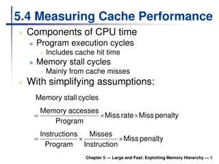
Cache Abstraction and Metrics Address Data Store Tag Store (stores memory blocks) (is the address in the cache? + bookkeeping) Hit/miss? Data Cache hit rate = (# hits) / (# hits + # misses) = (# hits) / (# accesses) Average memory access time (AMAT) = ( hit-rate * hit-latency ) + ( miss-rate * miss-latency ) Aside: Can reducing AMAT reduce performance? 35
A Basic Hardware Cache Design We will start with a basic hardware cache design Then, we will examine a multitude of ideas to make it better 36
Blocks and Addressing the Cache Memory is logically divided into fixed-size blocks Each block maps to a location in the cache, determined by the index bits in the address used to index into the tag and data stores tag index byte in block 3 bits 3 bits 2b Cache access: 1) index into the tag and data stores with index bits in address 2) check valid bit in tag store 3) compare tag bits in address with the stored tag in tag store 8-bit address If a block is in the cache (cache hit), the stored tag should be valid and match the tag of the block 37
Direct-Mapped Cache: Placement and Access Assume byte-addressable memory: 256 bytes, 8- byte blocks 32 blocks Assume cache: 64 bytes, 8 blocks Direct-mapped: A block can go to only one location tag index byte in block Data store Tag store 3 bits 3 bits 2b Address tag V byte in block =? MUX Hit? Data Addresses with same index contend for the same location: Cause conflict misses 38
Direct-Mapped Caches Direct-mapped cache: Two blocks in memory that map to the same index in the cache cannot be present in the cache at the same time One index one entry Can lead to 0% hit rate if more than one block accessed in an interleaved manner map to the same index Assume addresses A and B have the same index bits but different tag bits A, B, A, B, A, B, A, B, conflict in the cache index All accesses are conflict misses 39
Set Associativity Addresses 0 and 8 always conflict in direct mapped cache Instead of having one column of 8, have 2 columns of 4 blocks Tag store Data store SET tag tag V V =? =? MUX byte in block Logic MUX Hit? Address tag index byte in block Key idea: Associative memory within the set + Accommodates conflicts better (fewer conflict misses) -- More complex, slower access, larger tag store 2 bits 3 bits 3b 40
Higher Associativity 4-way Tag store =? =? =? =? Hit? Logic Data store MUX byte in block MUX + Likelihood of conflict misses even lower -- More tag comparators and wider data mux; larger tags 41
Full Associativity Fully associative cache A block can be placed in any cache location Tag store =? =? =? =? =? =? =? =? Logic Hit? Data store MUX byte in block MUX 42
Associativity (and Tradeoffs) Degree of associativity: How many blocks can map to the same index (or set)? Higher associativity ++ Higher hit rate -- Slower cache access time (hit latency and data access latency) -- More expensive hardware (more comparators) hit rate Diminishing returns from higher associativity associativity 43
Issues in Set-Associative Caches Think of each block in a set having a priority Indicating how important it is to keep the block in the cache Key issue: How do you determine/adjust block priorities? There are three key decisions in a set: Insertion, promotion, eviction (replacement) Insertion: What happens to priorities on a cache fill? Where to insert the incoming block, whether or not to insert the block Promotion: What happens to priorities on a cache hit? Whether and how to change block priority Eviction/replacement: What happens to priorities on a cache miss? Which block to evict and how to adjust priorities 44
Eviction/Replacement Policy Which block in the set to replace on a cache miss? Any invalid block first If all are valid, consult the replacement policy Random FIFO Least recently used (how to implement?) Not most recently used Least frequently used? Least costly to re-fetch? Why would memory accesses have different cost? Hybrid replacement policies Optimal replacement policy? 45
Implementing LRU Idea: Evict the least recently accessed block Problem: Need to keep track of access ordering of blocks Question: 2-way set associative cache: What do you need to implement LRU perfectly? Question: 4-way set associative cache: What do you need to implement LRU perfectly? How many different orderings possible for the 4 blocks in the set? How many bits needed to encode the LRU order of a block? What is the logic needed to determine the LRU victim? 46
Approximations of LRU Most modern processors do not implement true LRU (also called perfect LRU ) in highly-associative caches Why? True LRU is complex LRU is an approximation to predict locality anyway (i.e., not the best possible cache management policy) Examples: Not MRU (not most recently used) Hierarchical LRU: divide the N-way set into M groups , track the MRU group and the MRU way in each group Victim-NextVictim Replacement: Only keep track of the victim and the next victim 47
Hierarchical LRU (not MRU) Divide a set into multiple groups Keep track of only the MRU group Keep track of only the MRU block in each group On replacement, select victim as: A not-MRU block in one of the not-MRU groups (randomly pick one of such blocks/groups) 48
Cache Replacement Policy: LRU or Random LRU vs. Random: Which one is better? Example: 4-way cache, cyclic references to A, B, C, D, E 0% hit rate with LRU policy Set thrashing: When the program working set in a set is larger than set associativity Random replacement policy is better when thrashing occurs In practice: Depends on workload Average hit rate of LRU and Random are similar Best of both Worlds: Hybrid of LRU and Random How to choose between the two? Set sampling See Qureshi et al., A Case for MLP-Aware Cache Replacement, ISCA 2006. 49
What Is the Optimal? Belady s OPT Replace the block that is going to be referenced furthest in the future by the program Belady, A study of replacement algorithms for a virtual- storage computer, IBM Systems Journal, 1966. How do we implement this? Simulate? Is this optimal for minimizing miss rate? Is this optimal for minimizing execution time? No. Cache miss latency/cost varies from block to block! Two reasons: Remote vs. local caches and miss overlapping Qureshi et al. A Case for MLP-Aware Cache Replacement, ISCA 2006. 50


")

 Memory System")


")
")


")


")