Understanding Fill Area Primitives in Computer Graphics
An overview of fill area primitives in computer graphics, including the concept of fill areas, polygon fill areas, and polygon classifications into convex and concave polygons. This module covers the efficient processing of polygons, approximating curved surfaces, and generating wire-frame views of fill area shapes.

Download Presentation

Please find below an Image/Link to download the presentation.
The content on the website is provided AS IS for your information and personal use only. It may not be sold, licensed, or shared on other websites without obtaining consent from the author. Download presentation by click this link. If you encounter any issues during the download, it is possible that the publisher has removed the file from their server.
E N D
Presentation Transcript
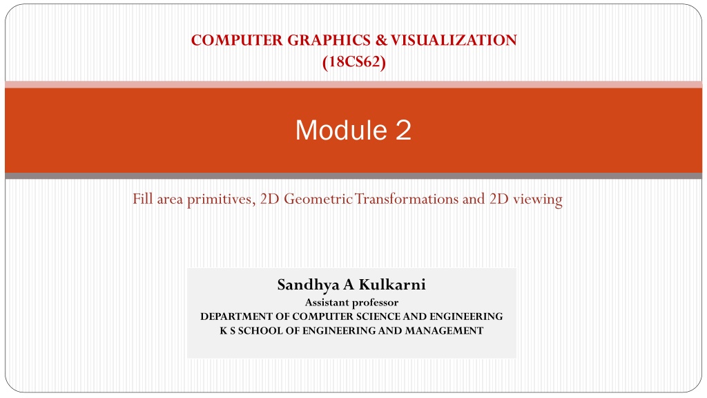
COMPUTER GRAPHICS & VISUALIZATION (18CS62) Module 2 Fill area primitives, 2D Geometric Transformations and 2D viewing Sandhya A Kulkarni Assistant professor DEPARTMENT OF COMPUTER SCIENCE AND ENGINEERING K S SCHOOL OF ENGINEERING AND MANAGEMENT
Fill-Area Primitives An useful construct for describing components of a picture is an area that is filled with some solid color or pattern. A picture component of this type is typically referred to as a fill area or a filled area. Any fill-area shape is possible, graphics libraries generally do not support specifications for arbitrary fill shapes Graphics routines can more efficiently process polygons than other kinds of fill shapes because polygon boundaries are described with linear equations. When lighting effects and surface-shading procedures are applied, an approximated curved surface can be displayed quite realistically. Approximating a curved surface with polygon facets is sometimes referred to as surface tessellation, or fitting the surface with a polygon mesh. Below figure shows the side and top surfaces of a metal cylinder approximated in an outline form as a polygon mesh.
Few possible fill-area shapes Displays of such figures can be generated quickly as wire-frame views, showing only the polygon edges to give a general indication of the surface structure Objects described with a set of polygon surface patches are usually referred to as standard graphics objects, or just graphics objects.
Polygon Fill Areas A polygon is a plane figure specified by a set of three or more coordinate positions, called vertices, that are connected in sequence by straight-line segments, called the edges or sides of the polygon. It is required that the polygon edges have no common point other than their endpoints. Thus, by definition, a polygon must have all its vertices within a single plane and there can be no edge crossings Examples of polygons include triangles, rectangles, octagons, and decagons Any plane figure with a closed-polyline boundary is alluded to as a polygon, and one with no crossing edges is referred to as a standard polygon or a simple polygon
Polygon Classifications Polygons are classified into two types 1. Convex Polygon and 2. Concave Polygon Convex Polygon: The polygon is convex if all interior angles of a polygon are less than or equal to 180 , where an interior angle of a polygon is an angle inside the polygon boundary that is formed by two adjacent edges An equivalent definition of a convex polygon is that its interior lies completely on one side of the infinite extension line of any one of its edges. Also, if we select any two points in the interior of a convex polygon, the line segment joining the two points is also in the interior. Concave Polygon: A polygon that is not convex is called a concave polygon, whose interior angle is > 180 Figures shows convex and concave polygon
Splitting a Convex Polygon into a Set of Triangles Once we have a vertex list for a convex polygon, we could transform it into a set of triangles. First define any sequence of three consecutive vertices to be a new polygon (a triangle). The middle triangle vertex is then deleted from the original vertex list . The same procedure is applied to this modified vertex list to strip off another triangle. We continue forming triangles in this manner until the original polygon is reduced to just three vertices, which define the last triangle in the set. Concave polygon can also be divided into a set of triangles using this approach, although care must be taken that the new diagonal edge formed by joining the first and third selected vertices does not cross the concave portion of the polygon, and that the three selected vertices at each step form an interior angle that is less than 180
Identifying Concave Polygons Characteristics: A concave polygon has at least one interior angle greater than 180 . The extension of some edges of a concave polygon will intersect other edges, and Some pair of interior points will produce a line segment that intersects the polygon boundary
Identification algorithm 1 Identifying a concave polygon by calculating cross-products of successive pairs of edge vectors. If we set up a vector for each polygon edge, then we can use the cross-product of adjacent edges to test for concavity. All such vector products will be of the same sign (positive or negative) for a convex polygon. Therefore, if some cross-products yield a positive value and some a negative value, we have a concave polygon
Identification algorithm 2 Look at the polygon vertex positions relative to the extension line of any edge. If some vertices are on one side of the extension line and some vertices are on the other side, the polygon is concave. Splitting Concave Polygons Split concave polygon it into a set of convex polygons using edge vectors and edge cross products; or, we can use vertex positions relative to an edge extension line to determine which vertices are on one side of this line and which are on the other.
Cross product Example: The cross product of a = (2,3,4) and b = (5,6,7) cx= aybz azby= 3 7 4 6 = 3 cy= azbx axbz= 4 5 2 7 = 6 cz= axby aybx= 2 6 3 5 = 3 Answer:a b = ( 3,6, 3)
1.Vector method First need to form the edge vectors. Given two consecutive vertex positions, Vk and Vk+1, we define the edge vector between them as Ek = Vk+1 Vk Calculate the cross-products of successive edge vectors in order around the polygon perimeter. If the z component of some cross-products is positive while other cross-products have a negative z component, the polygon is concave. We can apply the vector method by processing edge vectors in counterclockwise order If any cross- product has a negative z component (as in below figure), the polygon is concave and we can split it along the line of the first edge vector in the cross-product pair E1 = (1, 0, 0) E2 = (1, 1, 0) E3 = (1, 1, 0) E6 = (0, 2, 0) E4 = (0, 2, 0) E5 = ( 3, 0, 0)
Given : E1 = (1, 0, 0) E2 = (1, 1, 0) E3 = (1, 1, 0) E4 = (0, 2, 0) E5 = ( 3, 0, 0) E6 = (0, 2, 0) cx= aybz azby , cy= azbx axbz , cz= axby aybx E1 E2 =(0 0) - (0 1) =0 = (0 1) - (1 0) = 0 = (1 1) - (0 1) = 1 = (0, 0, 1) E2 E3 = (1 0) - (0 -1) = 0 = (0 1) - (1 0) = 0 = (1 -1) - (1 1) = -2 = (0, 0, -2)
The values for the above figure is as follows: E1 E2 = (0, 0, 1) E2 E3 = (0, 0, 2) E3 E4 = (0, 0, 2) E4 E5 = (0, 0, 6) E5 E6 = (0, 0, 6) E6 E1 = (0, 0, 2) Since the cross-product E2 E3 has a negative z component, we split the polygon along the line of vector E2. The line equation for this edge has a slope of 1 and a y intercept of 1 . No other edge cross-products are negative, so the two new polygons are both convex.
2. Rotational method Proceeding counterclockwise around the polygon edges, we shift the position of the polygon so that each vertex Vk in turn is at the coordinate origin. We rotate the polygon about the origin in a clockwise direction so that the next vertex Vk+1 is on the x axis. If the following vertex, Vk+2, is below the x axis, the polygon is concave. We then split the polygon along the x axis to form two new polygons, and we repeat the concave test for each of the two new polygons
Identifying interior and exterior region of polygon We may want to specify a complex fill region with intersecting edges. For such shapes, it is not always clear which regions of the xy plane we should call interior and which regions. We should designate as exterior to the object boundaries. Two commonly used algorithms 1. Odd-Even rule (Inside-Outside test) and 2. The nonzero winding-number rule.
1.Inside 1.Inside- -Outside Tests Outside Tests Also called the odd-parity rule or the even-odd rule. Draw a line from any position P to a distant point outside the coordinate extents of the closed polyline. Then we count the number of line-segment crossings along this line. If the number of segments crossed by this line is odd, then P is considered to be an interior point Otherwise, P is an exterior point We can use this procedure, for example, to fill the interior region between two concentric circles or two concentric polygons with a specified color.
2.Nonzero Winding 2.Nonzero Winding- -Number rule Number rule This counts the number of times that the boundary of an object winds around a particular point in the counterclockwise direction termed as winding number, Initialize the winding number to 0 and again imagining a line drawn from any position P to a distant point beyond the coordinate extents of the object. The line we choose must not pass through any endpoint coordinates. As we move along the line from position P to the distant point, we count the number of object line segments that cross the reference line in each direction We add 1 to the winding number every time we intersect a segment that crosses the line in the direction from right to left, and we subtract 1 every time we intersect a segment that crosses from left to right If the winding number is nonzero, P is considered to be an interior. Otherwise, P is taken to be an exterior point
Variation Variations of the nonzero winding-number rule can be used to define interior regions in other ways define a point to be interior if its winding number is positive or if it is negative; or we could use any other rule to generate a variety of fill shapes Boolean operations are used to specify a fill area as a combination of two regions One way to implement Boolean operations is by using a variation of the basic winding-number rule consider the direction for each boundary to be counterclockwise, the union of two regions would consist of those points whose winding number is positive The intersection of two regions with counterclockwise boundaries would contain those points whose winding number is greater than 1, To set up a fill area that is the difference of two regions (say, A B), we can enclose region A with a counterclockwise border and B with a clockwise border
Polygon Tables Polygon Tables The objects in a scene are described as sets of polygon surface facets The description for each object includes coordinate information specifying the geometry for the polygon facets and other surface parameters such as color, transparency, and light reflection properties. The data of the polygons are placed into tables that are to be used in the subsequent processing, display, and manipulation of the objects in the scene These polygon data tables can be organized into two groups: 1. Geometric tables and 2. Attribute tables Geometric data tables contain vertex coordinates and parameters to identify the spatial orientation of the polygon surfaces. Geometric data for the objects in a scene are arranged conveniently in three lists. 1. A Vertex Table: Stores Coordinate values for each vertex in the object. 2. A Edge Table: Contains pointers back into the vertex table to identify the vertices for each polygon edge. 3. A Surface-facet table: Contains pointers back into the edge table to identify the edges for each polygon Attribute information Tables for an object includes parameters specifying the degree of transparency of the object and its surface reflectivity and texture characteristics
Variations: The object can be displayed efficiently by using data from the edge table to identify polygon boundaries. 1. An alternative arrangement is to use just two tables: a vertex table and a surface-facet table this scheme is less convenient, and some edges could get drawn twice in a wireframe display. 2. Another possibility is to use only a surface-facet table, but this duplicates coordinate information, since explicit coordinate values are listed for each vertex in each polygon facet. Also the relationship between edges and facets would have to be reconstructed from the vertex listings in the surface-facet table. 3. We could expand the edge table to include forward pointers into the surface-facet table so that a common edge between polygons could be identified more rapidly the vertex table could be expanded to reference corresponding edges, for faster information retrieval
Tests for consistency and completeness Because the geometric data tables may contain extensive listings of vertices and edges for complex objects and scenes, it is important that the data be checked for consistency and completeness. Some of the tests that could be performed by a graphics package are 1. that every vertex is listed as an endpoint for at least two edges, 2. that every edge is part of at least one polygon, 3. that every polygon is closed, 4. that each polygon has at least one shared edge, and 5. that if the edge table contains pointers to polygons, every edge referenced by a polygon pointer has a reciprocal pointer back to the polygon.
OpenGL Polygon Fill-Area Functions A glVertex function is used to input the coordinates for a single polygon vertex, and a complete polygon is described with a list of vertices placed between a glBegin/glEnd pair. By default, a polygon interior is displayed in a solid color, determined by the current color settings we can fill a polygon with a pattern and we can display polygon edges as line borders around the interior fill. There are six different symbolic constants that we can use as the argument in the glBegin function to describe polygon fill areas In some implementations of OpenGL, the following routine can be more efficient than generating a fill rectangle using glVertex specifications: glRect* (x1, y1, x2, y2); One corner of this rectangle is at coordinate position (x1, y1), and the opposite corner of the rectangle is at position (x2, y2). Suffix codes for glRect specify the coordinate data type and whether coordinates are to be expressed as array elements. These codes are i (for integer), s (for short), f (for float), d (for double), and v (for vector). Example glRecti (200, 100, 50, 250); If we put the coordinate values for this rectangle into arrays, we can generate the same square with the following code: int vertex1 [ ] = {200, 100}; int vertex2 [ ] = {50, 250}; glRectiv (vertex1, vertex2);
1. Polygon With the OpenGL primitive constant GL POLYGON, we can display a single polygon fill area. Each of the points is represented as an array of (x, y) coordinate values: glBegin (GL_POLYGON); glVertex2iv (p1); glVertex2iv (p2); glVertex2iv (p3); glVertex2iv (p4); glVertex2iv (p5); glVertex2iv (p6); glEnd ( ); A polygon vertex list must contain at least three vertices. Otherwise, nothing is displayed. A single convex polygon fill area generated with the primitive constant GL POLYGON.
2. Triangles Displays the trianlges. Three primitives in triangles, GL_TRIANGLES, GL_TRIANGLE_FAN, GL_TRIANGLE_STRIP glBegin (GL_TRIANGLES); glVertex2iv (p1); glVertex2iv (p2); glVertex2iv (p6); glVertex2iv (p3); glVertex2iv (p4); glVertex2iv (p5); glEnd ( ); Two unconnected triangles generated with GL_TRIANGLES In this case, the first three coordinate points define the vertices for one triangle, the next three points define the next triangle, and so forth. For each triangle fill area, we specify the vertex positions in a counterclockwise order triangle strip
2.1 Assuming that no coordinate positions are repeated in a list of N vertices, we obtain N 2 triangles in the strip. Clearly, we must have N 3 or nothing is displayed. Each successive triangle shares an edge with the previously defined triangle, so the ordering of the vertex list must be set up to ensure a consistent display. 1. First triangle (n = 1) would be listed as having vertices (p1, p2, p6). 2. Second triangle (n = 2) would have vertex ordering (p6, p2, p3). 3. Third triangle (n = 3) would have vertex ordering (p6, p3, p5). 4. Fourth triangle (n = 4) would be listed in the polygon tables with vertex ordering (p5, p3, p4). Four connected triangles generated with GL TRIANGLE STRIP. glBegin (GL_TRIANGLE_STRIP); glVertex2iv (p1); glVertex2iv (p2); glVertex2iv (p6); glVertex2iv (p3); glVertex2iv (p5); glVertex2iv (p4); glEnd ( );
2.2 Another way to generate a set of connected triangles is to use the fan Approach glBegin (GL_TRIANGLE_FAN); glVertex2iv (p1); glVertex2iv (p2); glVertex2iv (p3); glVertex2iv (p4); glVertex2iv (p5); glVertex2iv (p6); glEnd ( ); For N vertices, we again obtain N 2 triangles, providing no vertex positions are repeated, and we must list at least three vertices be specified in the proper order to define front and back faces for each triangle correctly. 1. Triangle 1 is defined with the vertex list (p1, p2, p3); 2. Triangle 2 has the vertex ordering (p1, p3, p4); 3. Triangle 3 has its vertices specified in the order (p1, p4, p5); 4. Triangle 4 is listed with vertices (p1, p5, p6). Four connected triangles generated with GL TRIANGLE FAN.
3. OpenGL provides for the specifications of two types of quadrilaterals. With the GL QUADS primitive constant and the following list of eight vertices, specified as two-dimensional coordinate arrays, we can generate the display shown in Figure (a): glBegin (GL_QUADS); glVertex2iv (p1); glVertex2iv (p2); glVertex2iv (p3); glVertex2iv (p4); glVertex2iv (p5); glVertex2iv (p6); glVertex2iv (p7); glVertex2iv (p8); glEnd ( ); Quadrilaterals
3.1 Rearranging the vertex list in the previous quadrilateral code example and changing the primitive constant to GL_QUAD_STRIP, we can obtain the set of connected quadrilaterals: glBegin (GL_QUAD_STRIP); glVertex2iv (p1); glVertex2iv (p2); glVertex2iv (p4); glVertex2iv (p3); glVertex2iv (p5); glVertex2iv (p6); glVertex2iv (p8); glVertex2iv (p7); glEnd ( ); For a list of N vertices, we obtain N/2 1 quadrilaterals, providing that N 4. Thus, 1. First quadrilateral (n = 1) is listed as having a vertex ordering of (p1, p2, p3, p4). 2. Second quadrilateral (n=2) has the vertex ordering (p4, p3, p6, p5). 3. Third quadrilateral (n=3) has the vertex ordering (p5, p6, p7, p8). GL_QUAD_STRIP
Fill-Area Attributes We can fill any specified regions, including circles, ellipses, and other objects with curved boundaries Fill Styles A basic fill-area attribute provided by a general graphics library is the display style of the interior. We can display a region with a single color, a specified fill pattern, or in a hollow style by showing only the boundary of the region We can also fill selected regions of a scene using various brush styles, color-blending combinations, or textures.
For polygons, we could show the edges in different colors, widths, and styles; and we can select different display attributes for the front and back faces of a region. Fill patterns can be defined in rectangular color arrays that list different colors for different positions in the array. An array specifying a fill pattern is a mask that is to be applied to the display area. The mask is replicated in the horizontal and vertical directions until the display area is filled with non overlapping copies of the pattern. This process of filling an area with a rectangular pattern is called tiling, and a rectangular fill pattern is sometimes referred to as a tiling pattern predefined fill patterns are available in a system, such as the hatch fill patterns Hatch fill could be applied to regions by drawing sets of line segments to display either single hatching or cross hatching
Color-Blended Fill Regions Color-blended regions can be implemented using either transparency factors to control the blending of background and object colors, or using simple logical or replace operations as shown in figure The linear soft-fill algorithm repaints an area that was originally painted by merging a foreground color F with a single background color B, where F != B.
General Scan-Line Polygon-Fill Algorithm A scan-line fill of a region is performed by first determining the intersection positions of the boundaries of the fill region with the screen scan lines. Then the fill colors are applied to each section of a scan line that lies within the interior of the fill region. The simplest area to fill is a polygon, because each scanline intersection point with a polygon boundary is obtained by solving a pair of simultaneous linear equations, where the equation for the scan line is simply y = constant.
Figure above illustrates the basic scan-line procedure for a solid-color fill of a polygon. For each scan line that crosses the polygon, the edge intersections are sorted from left to right, and then the pixel positions between, and including, each intersection pair are set to the specified fill color the fill color is applied to the five pixels from x = 10 to x = 14 and to the seven pixels from x = 18 to x = 24.
Whenever a scan line passes through a vertex, it intersects two polygon edges at that point. In some cases, this can result in an odd number of boundary intersections for a scan line. Scan line y intersects an even number of edges, and the two pairs of intersection points along this scan line correctly identify the interior pixel spans. But scan line y intersects five polygon edges. Thus, as we process scan lines, we need to distinguish between these cases. For scan line y, the two edges sharing an intersection vertex are on opposite sides of the scan line. But for scan line y , the two intersecting edges are both above the scan line.
Thus, a vertex that has adjoining edges on opposite sides of an intersecting scan line should be counted as just one boundary intersection point. If the three endpoint y values of two consecutive edges monotonically increase or decrease, we need to count the shared (middle) vertex as a single intersection point for the scan line passing through that vertex. Otherwise, the shared vertex represents a local extremum (minimum or maximum) on the polygon boundary, and the two edge intersections with the scan line passing through that vertex can be added to the intersection list. One method for implementing the adjustment to the vertex-intersection count is to shorten some polygon edges to split those vertices that should be counted as one intersection. We can process non horizontal edges around the polygon boundary in the order specified, either clockwise or counterclockwise.
Adjusting endpoint y values for a polygon, as we process edges in order around the polygon perimeter. The edge currently being processed is indicated as a solid line In (a), the y coordinate of the upper endpoint of the current edge is decreased by 1. In (b), the y coordinate of the upper endpoint of the next edge is decreased by 1. Coherence properties can be used in computer-graphics algorithms to reduce processing. Coherence methods often involve incremental calculations applied along a single scan line or between successive scan lines
The slope of this edge can be expressed in terms of the scan- line intersection coordinates: Because the change in y coordinates between the two scan lines is simply y k+1 yk= 1 The x-intersection value xk+1 on the upper scan line can be determined from the x intersection value xk on the preceding scan line as Each successive x intercept can thus be calculated by adding the inverse of the slope and rounding to the nearest integer.
Along an edge with slope m, the intersection xk value for scan line k above the initial scan line can be calculated as xk= x0 +k/m Where, m is the ratio of two integers Where x and y are the differences between the edge endpoint x and y coordinate values. Thus, incremental calculations of x intercepts along an edge for successive scan lines can be expressed as
To perform a polygon fill efficiently, we can first store the polygon boundary in a sorted edge table that contains all the information necessary to process the scan lines efficiently. Proceeding around the edges in either a clockwise or a counterclockwise order, we can use a bucket sort to store the edges, sorted on the smallest y value of each edge, in the correct scan-line positions. Only non horizontal edges are entered into the sorted edge table. Each entry in the table for a particular scan line contains the maximum y value for that edge, the x-intercept value (at the lower vertex) for the edge, and the inverse slope of the edge. For each scan line, the edges are in sorted order from left to right We process the scan lines from the bottom of the polygon to its top, producing an active edge listfor each scan line crossing the polygon boundaries. The active edge list for a scan line contains all edges crossed by that scan line, with iterative coherence calculations used to obtain the edge intersections Implementation of edge-intersection calculations can be facilitated by storing x and y values in the sorted edge list
Each entry in the table for a particular scan line contains the maximum y value for that edge, the x-intercept value (at the lower vertex) for the edge, and the inverse slope of the edge.
Plane Equations Each polygon in a scene is contained within a plane of infinite extent. The general equation of a plane is Ax + By + Cz + D = 0 Where, 1. (x, y, z) is any point on the plane, and 2. The coefficients A, B, C, and D (called plane parameters) are constants describing the spatial properties of the plane. We can obtain the values of A, B, C, and D by solving a set of three plane equations using the coordinate values for three non collinear points in the plane for the three successive convex-polygon vertices, (x1, y1, z1), (x2, y2, z2), and (x3, y3, z3), in a counterclockwise order and solve the following set of simultaneous linear plane equations for the ratios A/D, B/D, and C/D: (A/D)xk + (B/D)yk + (C/D)zk= 1, k = 1, 2, 3
The solution to this set of equations can be obtained in determinant form, using Cramer s rule, as Expanding the determinants, we can write the calculations for the plane coefficients in the form
Problem: It is possible that the coordinates defining a polygon facet may not be contained within a single plane. Solution: We can solve this problem by 1. dividing the facet into a set of triangles; 2. or we could find an approximating plane for the vertex list. Obtaining an approximating plane is to 1. divide the vertex list into subsets, where each subset contains three vertices, 2. and calculate plane parameters A, B, C, D for each subset.
Front and Back Polygon Faces The side of a polygon that faces into the object interior is called the back face, and the visible, or outward, side is the front face . Every polygon is contained within an infinite plane that partitions space into two regions. 1. Any point that is not on the plane and that is visible to the front face of a polygon surface section is said to be in front of (or outside) the plane, and, thus, outside the object. 2. And any point that is visible to the back face of the polygon is behind (or inside) the plane. Plane equations can be used to identify the position of spatial points relative to the polygon facets of an object.
For any point (x, y, z) not on a plane with parameters A, B, C, D, we have Ax + By + Cz + D != 0 Thus, we can identify the point as either behind or in front of a polygon surface contained within that plane according to the sign (negative or positive) of Ax + By + Cz + D: if Ax + B y + C z + D < 0, the point (x, y, z) is behind the plane if Ax + B y + C z + D > 0, the point (x, y, z) is in front of the plane
Orientation of a polygon surface in space can be described with the normal vector for the plane containing that polygon The normal vector points in a direction from inside the plane to the outside; that is, from the back face of the polygon to the front face. Thus, the normal vector for this plane is N = (1, 0, 0), which is in the direction of the positive x axis. That is, the normal vector is pointing from inside the cube to the outside and is perpendicular to the plane x = 1. The elements of a normal vector can also be obtained using a vector cross product Calculation.
We have a convex-polygon surface facet and a right-handed Cartesian system, we again select any three vertex positions,V1,V2, and V3, taken in counterclockwise order when viewing from outside the object toward the inside. Forming two vectors, one from V1 to V2 and the second from V1 to V3, we calculate N as the vector cross-product: N = (V2 V1) (V3 V1) This generates values for the plane parameters A, B, and C.We can then obtain the value for parameter D by substituting these values and the coordinates in Ax + B y + C z + D = 0 The plane equation can be expressed in vector form using the normal N and the position P of any point in the plane as N P = D


 not on a plane with parameters")