Lower Bounds for Small Depth Arithmetic Circuits
This work explores lower bounds for small-depth arithmetic circuits, jointly conducted by researchers from MSRI, IITB, and experts in the field. They investigate the complexity of multivariate polynomials in arithmetic circuits, discussing circuit depth, size, and the quest for an explicit family of n-variate polynomials with super-polynomial circuit size requirements. The study delves into questions about the explicitness of polynomial families such as the Permanent and their degrees.

Download Presentation

Please find below an Image/Link to download the presentation.
The content on the website is provided AS IS for your information and personal use only. It may not be sold, licensed, or shared on other websites without obtaining consent from the author. Download presentation by click this link. If you encounter any issues during the download, it is possible that the publisher has removed the file from their server.
E N D
Presentation Transcript
Lower bounds for small depth arithmetic circuits Joint work with Neeraj Kayal (MSRI) Nutan Limaye (IITB) Srikanth Srinivasan (IITB) Chandan Saha
Arithmetic Circuit: A model of computation f(x1, x2, , xn) --> multivariate polynomial in x1, , xn gh + x h g x x x x Product gate g+h + + + + . + x x x x h g Sum gate .. x1 x2 xn-1 xn There are `field constants on the wires
Arithmetic Circuit: A model of computation f(x1, x2, , xn) + x x x x Depth = 4 + + + + . x x x x .. x1 x2 xn-1 xn
Arithmetic Circuit: A model of computation f(x1, x2, , xn) + x x x x Size = no. of gates and wires + + + + . x x x x .. x1 x2 xn-1 xn
The lower bound question Is there an explicit family of n-variate, poly(n) degree polynomials {fn} that requires super-polynomial in n circuit size ?
The lower bound question Is there an explicit family of n-variate, poly(n) degree polynomials {fn} that requires super-polynomial in n circuit size ? Note : A random polynomial has super-poly(n) circuit size
The Permanent an explicit family Permn = xi (i) Sn i [n]
The Permanent an explicit family Permn = xi (i) Sn i [n] Degree of Permn is low. i.e. bounded by poly(n)
The Permanent an explicit family Permn = xi (i) Sn i [n] Degree of Permn is low. Coefficient of any given monomial can be found efficiently. given a monomial, there s a poly-time algorithm to determine the coefficient of the monomial.
The Permanent an explicit family Permn = xi (i) Sn i [n] Degree of Permn is low. These two properties characterize explicitness Coefficient of any given monomial can be found efficiently.
The Permanent an explicit family Permn = xi (i) Sn i [n] Degree of Permn is low. Define class VNP Coefficient of any given monomial can be found efficiently.
The Permanent an explicit family Permn = xi (i) Sn i [n] Degree of Permn is low. Define class VNP Coefficient of any given monomial can be found efficiently. Class VP: Contains families of low degree polynomials {fn} that can be computed by poly(n)-size circuits.
The Permanent an explicit family Permn = xi (i) Sn i [n] Degree of Permn is low. Coefficient of any given monomial can be found efficiently. VP vs VNP: Does Permn family require super-poly(n) size circuits?
A strategy for proving arithmetic circuit lower bound Step 1: Depth reduction Step 2: Lower bound for small depth circuits
A strategy for proving arithmetic circuit lower bound Step 1: Depth reduction Step 2: Lower bound for small depth circuits
Notations and Terminologies Notations: n = no. of variables in fn d = degree bound on fn = nO(1) Homogeneous polynomial: A polynomial is homogeneous if all its monomials have the same degree (say, d). Homogeneous circuits: A circuit is homogeneous if every gate outputs/computes a homogeneous polynomial. Multilinear polynomial: In every monomial, degree of every variable is at most 1.
Reduction to depth log d Valiant, Skyum, Berkowitz, Rackoff (1983). Homogeneous, degree d, fn computed by poly(n) circuit fn computed by homogeneous poly(n) circuit of depth O(log d) arbitrary depth log d poly(n) poly(n)
Reduction to depth 4 Agrawal, Vinay (2008); Koiran (2010); Tavenas (2013). Homogeneous, degree d, fn computed by poly(n) circuit fn computed by homogeneous depth 4 circuit of size nO( d) log d 4 nO( d) poly(n)
Reduction to depth 4 Agrawal, Vinay (2008); Koiran (2010); Tavenas (2013). Homogeneous, degree d, fn computed by poly(n) circuit fn computed by homogeneous depth 4 circuit of size nO( d) fn can have nO(d) monomials ! log d 4 nO( d) poly(n)
A depth 4 circuit + x x x x + + + + . x x x x .. x1 x2 xn-1 xn
A depth 4 circuit Qij i j + x x x x sum of monomials Qij + + + + . x x x x .. x1 x2 xn-1 xn
Reduction to depth 3 Gupta, Kamath, Kayal, Saptharishi (2013); Tavenas (2013). Homogeneous, degree d, fn computed by poly(n) circuit fn computed by depth 3 circuit of size nO( d) 4 3 nO( d) nO( d)
Reduction to depth 3 Gupta, Kamath, Kayal, Saptharishi (2013); Tavenas (2013). Homogeneous, degree d, fn computed by poly(n) circuit fn computed by depth 3 circuit of size nO( d) not homogeneous! 4 3 nO( d) nO( d)
A depth 3 circuit lij i j + x x x x linear polynomial lij + + + + . bottom fanin x1 x2 xn-1 xn
Implication of the depth reductions Let {fn} be an explicit family of polynomials. 4 if fn takes n ( d) size homogeneous VP VNP or if fn takes n ( d) size 3
A strategy for proving arithmetic circuit lower bound Step 1: Depth reduction Step 2: Lower bound for small depth circuits
Lower bound for homogeneous depth 4 Theorem: There is a family of homogeneous polynomials {fn} in VNP (with deg fn = d) such that any homogeneous depth-4 circuit computing fn has size n ( d) fn 4 size = n ( d)
Lower bound for homogeneous depth 4 Theorem: There is a family of homogeneous polynomials {fn} in VNP (with deg fn = d) such that any homogeneous depth-4 circuit computing fn has size n ( d) sum of monomials fn i Qij j fn = 4 size = n ( d) has size n ( d)
Lower bound for homogeneous depth 4 Theorem: There is a family of homogeneous polynomials {fn} in VNP (with deg fn = d) such that any homogeneous depth-4 circuit computing fn has size n ( d) fn 4 size = n ( d) joint work with Kayal, Limaye , Srinivasan
Lower bound for homogeneous depth 4 Theorem: There is a family of homogeneous polynomials {fn} in VNP (with deg fn = d) such that any homogeneous depth-4 circuit computing fn has size n ( d) fn 4 size = n ( d) the technique appears to be using homogeneity crucially
Lower bound for depth 3 Theorem: There is a family of homogeneous polynomials {fn} in VNP (with deg fn = d) such that any depth-3 circuit (bottom fanin d) computing fn has size n ( d) fn 3 size = n ( d)
Lower bound for depth 3 Theorem: There is a family of homogeneous polynomials {fn} in VNP (with deg fn = d) such that any depth-3 circuit (bottom fanin d) computing fn has size n ( d) needn t be homogeneous fn 3 size = n ( d)
Lower bound for depth 3 Theorem: There is a family of homogeneous polynomials {fn} in VNP (with deg fn = d) such that any depth-3 circuit (bottom fanin d) computing fn has size n ( d) fn Note: Even for bottom fanin d, depth-3 circuits n ( d) VP VNP 3 size = n ( d)
Lower bound for depth 3 Theorem: There is a family of homogeneous polynomials {fn} in VNP (with deg fn = d) such that any depth-3 circuit (bottom fanin t) computing fn has size n (d/t) fn 3 size = n (d/t) joint work with Kayal
Lower bound for depth 3 Theorem: There is a family of homogeneous polynomials {fn} in VNP (with deg fn = d) such that any depth-3 circuit (bottom fanin t) computing fn has size n (d/t) fn 3 size = n (d/t) answers a question by Shpilka & Wigderson (1999)
Complexity measure A measure is a function : F[x1, , xn] -> R. We wish to find a measure such that 1. If C is a circuit (say, a depth 4 circuit) then (C) s. small quantity , where s = size(C) Upper bound 2. For an explicit polynomial fn , (fn) large quantity Lower bound large quantity Implication: If C = fn then s small quantity
Some complexity measures Incomplete list ? Measure Model Partial derivatives (Nisan & Wigderson) homogeneous depth-3 circuits Evaluation dimension (Raz) multilinear formulas Hessian (Mignon & Ressayre) determinantal complexity permanent Jacobian (Agrawal et. al.) occur-k, depth-4 circuits
Some complexity measures Measure Model Partial derivatives (Nisan & Wigderson) homogeneous depth-3 circuits Evaluation dimension (Raz) multilinear formulas Hessian (Mignon & Ressayre) determinantal complexity permanent Jacobian (Agrawal et. al.) occur-k, depth-4 circuits Shifted partials (Kayal; Gupta et. al.) homog. depth-4 with low bottom fanin Projected shifted partials homogeneous depth-4 circuits; depth-3 circuits (with low bottom fanin)
Space of Partial Derivatives Notations: =k f : Set of all kth order derivatives of f(x1, , xn) < S > : The vector space spanned by F-linear combinations of polynomials in S Definition: PDk(f) = dim(< =k f >) Sub-additive property: PDk(f1 + f2) PDk(f1) + PDk(f2)
Space of Shifted Partials Notation: x= = Set of all monomials of degree SPk, (f) := dim (< x= . =k f >) Definition: Sub-additivity: SPk, (f1 + f2) SPk, (f1) + SPk, (f2)
Space of Shifted Partials Notation: x= = Set of all monomials of degree SPk, (f) := dim (< x= . =k f >) Definition: Sub-additivity: SPk, (f1 + f2) SPk, (f1) + SPk, (f2) Why do we expect SP(C) to be small ?
Shifted partials the intuition C = Q11Q12 Q1m+ + Qs1Qs2 Qsm(homog. depth 4) Qij = Sum of monomials
Shifted partials the intuition C = Q11Q12 Q1m+ + Qs1Qs2 Qsm(homog. depth 4) Observation: =k Qi1 Qimhas many roots if k << m << n any common root of Qi1 Qim is also a common root of =k Qi1 Qim
Shifted partials the intuition C = Q11Q12 Q1m+ + Qs1Qs2 Qsm(homog. depth 4) Observation: Dimension of the variety of =k Qi1 Qim is large if k << m << n
Shifted partials the intuition C = Q11Q12 Q1m+ + Qs1Qs2 Qsm(homog. depth 4) Observation: Dimension of the variety of =k Qi1 Qim is large if k << m << n [Hilbert s] Theorem (informal): If dimension of the variety of {g} is large then dim (< x= . {g} >) is small.
Shifted partials the intuition C = Q11Q12 Q1m+ + Qs1Qs2 Qsm(homog. depth 4) Observation: Dimension of the variety of =k Qi1 Qim is large if k << m << n [Hilbert s] Theorem (informal): If dimension of the variety of {g} is large then dim (< x= . {g} >) is small. so we expect SPk, (Qi1 Qim) to be a `small quantity
Shifted partials the intuition C = Q11Q12 Q1m+ + Qs1Qs2 Qsm(homog. depth 4) Observation: Dimension of the variety of =k Qi1 Qim is large if k << m << n [Hilbert s] Theorem (informal): If dimension of the variety of {g} is large then dim (< x= . {g} >) is small. by subadditivity, SPk, (C) s . `small quantity
Depth-4 with low bottom degree C = Q11Q12 Q1m+ + Qs1Qs2 Qsm(homog. depth 4) Qij = Sum of monomials of degree t (w.l.o.g m 2d/t )