FIR Filter Design Examples in Digital Signal Processing

Explore various FIR filter design examples using different windowing techniques like rectangular, Bartlett, Hanning, Hamming, and Blackman in E&E-ENG course from Fall 2015. Learn about the design parameters, frequency response, and characteristics of each window function through detailed plots and explanations.

Download Presentation

Please find below an Image/Link to download the presentation.
The content on the website is provided AS IS for your information and personal use only. It may not be sold, licensed, or shared on other websites without obtaining consent from the author. Download presentation by click this link. If you encounter any issues during the download, it is possible that the publisher has removed the file from their server.
E N D
Presentation Transcript
FIR Filter Design Examples EMU E&E-ENG Fall 2015
M = 64; n = -M:M; w = -pi:0.02:pi wrect = [0 ones(1,127) 0]; wbartlet = 1- (abs(n)/(M+1)); whanning= 0.5*(1+ cos((2*pi*n/(2*M+1)))); whamming = 0.54 + 0.46*cos((2*pi*n/(2*M+1))); wblackman = 0.42+0.5*cos((2*pi*n/(2*M+1))) + 0.08*cos((4*pi*n/(2*M+1))); figure(1); plot(n,wrect,'r') hold on plot(n,wbartlet,'b') plot(n,whanning,'g') plot(n,whamming,'m') plot(n,wblackman,'k')
1 0.9 0.8 0.7 0.6 0.5 0.4 rectangular Bartlett(triangular) Hanning Hamming Bartlet 0.3 0.2 0.1 0 -80 -60 -40 -20 0 20 40 60 80
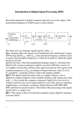
M = 64; n = -M:M; w = -pi:0.02:pi srect = sin((2*M+1)*w/2)./sin(w/2); sbartlet = 1/(M+1) * sin((2*M+1)*w/2)./sin(w/2); shanning = 0.5*srect + 0.25* (sin((2*M+1)*(w-(2*pi/(2*M+1)))/2)./sin((w-(2*pi/(2*M+1)))/2)) + 0.25* (sin((2*M+1)*(w+(2*pi/(2*M+1)))/2)./sin((w+(2*pi/(2*M+1)))/2)) ; shamming = 0.54*srect + 0.23* (sin((2*M+1)*(w-(2*pi/(2*M+1)))/2)./sin((w-(2*pi/(2*M+1)))/2)) + 0.23* (sin((2*M+1)*(w+(2*pi/(2*M+1)))/2)./sin((w+(2*pi/(2*M+1)))/2)) ; sblackman = 0.42*srect + 0.25* (sin((2*M+1)*(w-(2*pi/(2*M+1)))/2)./sin((w-(2*pi/(2*M+1)))/2)) + 0.25* (sin((2*M+1)*(w+(2*pi/(2*M+1)))/2)./sin((w+(2*pi/(2*M+1)))/2)) + 0.04* (sin((2*M+1)*(w- (4*pi/(2*M+1)))/2)./sin((w-(4*pi/(2*M+1)))/2)) + 0.04* (sin((2*M+1)*(w+(4*pi/(2*M+1)))/2)./sin((w+(4*pi/(2*M+1)))/2)) figure(2), plot(w,20*log10(abs(srect)),'r') hold on plot(w,20*log10(abs(sbartlet)),'b') plot(w,20*log10(abs(shanning)),'g') plot(w,20*log10(abs(shamming)),'m') plot(w,20*log10(abs(sblackman)),'k') legend('Rectangular','Bartlett','Hanning','Hamming','Blackman') grid on
60 Rectangular Bartlett Hanning Hamming Blackman 40 20 0 -20 -40 -60 -80 -100 -120 -140 -4 -3 -2 -1 0 1 2 3 4
Rectangular Bartlett Hanning Hamming Blackman 40 30 20 10 0 -10 -20 -30 -40 -50 -60 -0.6 -0.4 -0.2 0 0.2 0.4 0.6
MATLAB wp =0.5*pi; ws =0.35*pi; Ap=0.1; As=50; deltap = (10^(Ap/20)-1)/(10^(Ap/20)+1); deltas =(1+deltap)/(10^(As/20)); delta =min(deltap,deltas); A=round(-20*log10(delta)); Deltaw = wp-ws; omegac= (ws+wp)/2; M =ceil(6.6*pi/Deltaw); L=M+1; n=0:M;
h=hamming(L)'.*(omegac/pi).*sinc((omegac/pi)*(n-(M/2))); figure(1); [H,W]=freqz(h); Wlow = W(find(W<=wp)) ; NP = length(Wlow); Whigh = W(find(W>ws)); NS = length(Whigh); N=length(W); errp = abs(H(1:NP))-1; errs = abs(H(N-NS+1:N)); figure(2); plot(Wlow,errp,Whigh,errs);
50 Magnitude (dB) 0 -50 -100 -150 0 0.1 0.2 0.3 0.4 0.5 0.6 0.7 0.8 0.9 1 Normalized Frequency ( rad/sample) 0 Phase (degrees) -1000 -2000 -3000 0 0.1 0.2 0.3 0.4 0.5 0.6 0.7 0.8 0.9 1 Normalized Frequency ( rad/sample)
The advantage of the above adjustable windows in comparison to the fixed windows Are their near optimality and flexibility. Given ??, ??and the minimum stopband attenuation Asof the filter, the adjustable parameter (for Kaiser window) can be determined to give the desired value for As. Also M can be determined to give the desired value for the transition band ? = ?? ??of the filter.
Example: Consider the design of an FIR low-pass filter using a Kaiser window. The filter specifications are ??= 0.3? ,??= 0.4? and As= 50dB. ??+?? 2 ?? ?? 2? The cutoff frequency ??= = 0.35? Transition bandwidth ? = = 0.05 As= 50.00076dB = -20log10(??) ??= 0.0031622776 Then can be computed from the table in Table 4.5 = 4.533514 The filter order can be found using . 7 95 s A = N . 2 285 = 58.577377 . The next highest odd valued integer is N = 59
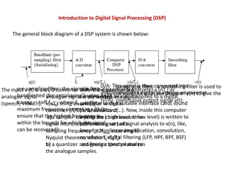
N=59 ; alpha = 4.5513; w = kaiser (N,alpha); disp('window coefficients') disp(w) [H,omega]= freqz(w); mag = 20*log10(abs(H)); figure; plot(omega/pi,mag); grid xlabel('Normalized Frequency') ylabel('Gain(dB)') title ('Lowpass filter using Kaiser window')
FT of the Kaiser Window 40 20 0 Gain(dB) -20 -40 -60 -80 0 0.1 0.2 0.3 0.4 0.5 0.6 0.7 0.8 0.9 1 Normalized Frequency
[n,wn,beta] = kaiserord([0.3 0.4]*pi,[1 0],[0.003162 hn = fir1(n,wn,kaiser(n+1,beta),'noscale'); figure; stem(hn) xlabel('Sample Number') ylabel('Amplitude') 0.003162],2*pi); >> n n = 59 >> beta beta = 4.5513
Specifications ??= 0.4?,??= 0.6?,?1= 0.01,?2= 0.001 Window design method assume Determine cut-off frequency Due to the symmetry we can choose it to be Compute = = 001 . 0 1 2 Type equation here. And Kaiser window parameters ? = 5.653 Then the impulse response is given as ? = 37
[n,wn,beta] = kaiserord([0.4 0.6]*pi,[1 0],[0.01 0.001],2*pi); hn = fir1(n,wn,kaiser(n+1,beta),'noscale'); figure; stem(hn) xlabel('Sample Number') ylabel('Amplitude') >> n n = 37 >> beta beta = 5.6533
0.6 0.5 0.4 0.3 Amplitude 0.2 0.1 0 -0.1 0 5 10 15 20 25 30 35 40 Sample Number
20 0 -20 -40 Gain(dB) -60 -80 -100 -120 0 0.1 0.2 0.3 0.4 0.5 0.6 0.7 0.8 0.9 1 Normalized Frequency


'.*(omegac/pi).*sinc((omegac/pi)*(n-(M/2)));")