Understanding Interpolation and Pulse Shaping in Real-Time Digital Signal Processing
Discrete-to-continuous conversion, interpolation, pulse shaping techniques, and data conversion in real-time digital signal processing are discussed in this content. Topics include types of pulse shapes, sampling, continuous signal approximation, interpolation methods, and data conversion processes from analog to digital and digital to analog. Concepts such as aliasing, pulse overlap, and different interpolation techniques like zero-order hold and linear interpolation are also covered.

Download Presentation

Please find below an Image/Link to download the presentation.
The content on the website is provided AS IS for your information and personal use only. It may not be sold, licensed, or shared on other websites without obtaining consent from the author. Download presentation by click this link. If you encounter any issues during the download, it is possible that the publisher has removed the file from their server.
E N D
Presentation Transcript
EE445S Real-Time Digital Signal Processing Lab Spring 2014 Interpolation and Pulse Shaping Prof. Brian L. Evans Dept. of Electrical and Computer Engineering The University of Texas at Austin Lecture 7
Outline Discrete-to-continuous conversion Interpolation Pulse shapes Rectangular Triangular Sinc Raised cosine Sampling and interpolation demonstration Conclusion 7 - 2
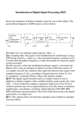
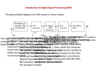
Data Conversion Analog-to-Digital Conversion Lowpass filter has stopband frequency less than fs to reduce aliasing due to sampling (enforce sampling theorem) Digital-to-Analog Conversion Discrete-to-continuous conversion could be as simple as sample and hold Lowpass filter has stopband frequency less than fs to reduce artificial high frequencies Lecture 4 Lecture 8 Analog Lowpass Filter Quantizer Sampler at sampling rate of fs Lecture 7 Discrete to Continuous Conversion Analog Lowpass Filter fs 7 - 3
Discrete-to-Continuous Conversion Input: sequence of samples y[n] Output: smooth continuous-time function obtained through interpolation (by connecting the dots ) [n y ] If f0 < fs , then ] [ = A n y ( ) + cos 2 f T n 3 4 5 6 7 0 s n would be converted to ~ = A t y ~t y 1 2 ( ) ( ) 0 + ( ) cos 2 t f Otherwise, aliasing has occurred, and the converter would reconstruct a cosine wave whose frequency is equal to the aliased positive frequency that is less than fs 7 - 4
Discrete-to-Continuous Conversion General form of interpolation is sum of weighted pulses = n ~ = ( ) [ ] ( sn T ) y t y n p t Sequence y[n] converted into continuous-time signal that is an approximation of y(t) Pulse function p(t) could be rectangular, triangular, parabolic, sinc, truncated sinc, raised cosine, etc. Pulses overlap in time domain when pulse duration is greater than or equal to sampling period Ts Pulses generally have unit amplitude and/or unit area Above formula is related to discrete-time convolution 7 - 5
Interpolation From Tables Using mathematical tables of numeric values of functions to compute a value of the function x 0 1 2 3 f(x) 0.0 1.0 4.0 9.0 Estimate f(1.5) from table Zero-order hold: take value to be f(1) to make f(1.5) = 1.0 ( stairsteps ) Linear interpolation: average values of nearest two neighbors to get f(1.5) = 2.5 Curve fitting: fit four points in table to polynomal a0 + a1x + a2x2 + a3x3 which gives f(1.5) = x2 = 2.25 ~x f ( ) 9 4 1 x 0 1 2 3 7 - 6
Rectangular Pulse Zero-order hold Easy to implement in hardware or software = 0 p(t) 1 1 t 1 if T t T 1 = ( ) rect p t s s 2 2 T otherwise s - Ts Ts t The Fourier transform is ( ) x sin( T ) sin f x ( ) = = = ( ) sinc T where sinc ( ) s P f T f T x s s s T f s In time domain, no overlap between p(t) and adjacent pulses p(t - Ts) and p(t + Ts) In frequency domain, sinc has infinite two-sided extent; hence, the spectrum is not bandlimited 7 - 7
Sinc Function ( ) x sin x ( ) x = sinc sinc(x) 1 How compute to sinc(0)? As numerator 0, and x x denominato both are r going 3 2 2 3 0 How 0. to handle to it? Even function (symmetric at origin) Zero crossings at Amplitude decreases proportionally to 1/x = , 2 , 3 ... , x 7 - 8
Triangular Pulse Linear interpolation It is relatively easy to implement in hardware or software, although not as easy as zero-order hold = otherwise 0 p(t) 1 | T | t 1 if T t T t = s s ( ) p t s T -Ts Ts t s Overlap between p(t) and its adjacent pulses p(t - Ts) and p(t + Ts) but with no others Fourier transform is How to compute this? Hint: Triangular pulse is equal to 1 / Ts times the convolution of rectangular pulse with itself In frequency domain, sinc2(fTs) has infinite two-sided extent; hence, the spectrum is not bandlimited ( ) = 2 ( ) sinc T P f T f s s 7 - 9
Sinc Pulse Ideal bandlimited interpolation sin t T 1 f 1 = = s = ( ) sinc p t t ( ) rect P f = W T T T 2 sT t s s s T s In time domain, infinite overlap between other pulses Fourier transform has extent f [-W, W], where P(f) is ideal lowpass frequency response with bandwidth W In frequency domain, sinc pulse is bandlimited Interpolate with infinite extent pulse in time? Truncate sinc pulse by multiplying it by rectangular pulse Causes smearing in frequency domain (multiplication in time domain is convolution in frequency domain) 7 - 10
Raised Cosine Pulse: Time Domain Pulse shaping used in communication systems ( ) 2 2 2 16 1 t W T s cos 2 t W t sinc = ( ) p t ideal lowpass filter impulse response Attenuation by 1/t2 for large t to reduce tail W is bandwidth of an ideal lowpass response [0, 1] rolloff factor Zero crossings at t = Ts , 2 Ts, See handout G in reader on raised cosine pulse 7 - 11
Raised Cosine Pulse Spectra Pulse shaping used in communication systems Bandwidth increased by factor of (1 + ): (1 + ) W = 2 W f1 f1 marks transition from passband to stopband 2W W f f P 1 1 | if 0 | f f = W 1 2 sT ( ) 1 | W | = ( ) 1 sin if | | 2 f f W f f1 1 1 4W 2 2 f = 1 1 W 0 otherwise Bandwidth generally scarce in communication systems 7 - 12
Sampling and Interpolation Demo DSP First, Ch. 4, Sampling and interpolation, http://www.ece.gatech.edu/research/DSP/DSPFirstCD/ Sample sinusoid y(t) to form y[n] Reconstruct sinusoid using rectangular, triangular, or truncated sinc pulse p(t) Which pulse gives the best reconstruction? Sinc pulse is truncated to be four sampling periods long. Why is the sinc pulse truncated? What happens as the sampling rate is increased? ~ = n = ( ) [ ] ( sn T ) y t y n p t 7 - 13
Conclusion Discrete-to-continuous time conversion involves interpolating between known discrete-time samples y[n] using pulse shape p(t) = n [n y ] ~ = ( ) [ ] ( sn T ) y t y n p t 3 4 5 6 7 n ~t y 1 2 Common pulse shapes Rectangular for same-and-hold interpolation Triangular for linear interpolation Sinc for optimal bandlimited linear interpolation but impractical Truncated raised cosine for practical bandlimited interpolation Truncation causes smearing in frequency domain ( ) 7 - 14