Distribution Feeder Modeling and Analysis Overview
 undefined

EE653 Power distribution system
modeling, optimization and
simulation
Dr. Zhaoyu Wang
1113 Coover Hall, Ames, IA
wzy@iastate.edu
ECpE Department
2
Distribution Feeder Modeling
and Analysis
Part I. High-Level Summary of
Distribution Feeder Modeling
Acknowledgement: The slides are developed based in part
on Distribution System Modeling and Analysis, 4
th
edition,
William H. Kersting, CRC Press, 2017
3
General Feeder Modeling - Series Components
•
A typical distribution feeder consists of the primary main with laterals tapped off the
primary main and sub-laterals tapped off the laterals.
•
A distribution feeder can be broken into the “series” components and the “shunt”
components. These series components can be lines, transformers, voltage regulators...
•
Fig. 2 is a general model of series component; no distinction is made as to what type of
element is connected between nodes.
Fig.1 A typical unbalanced distribution feeder
Fig.2 Standard feeder series component
model
ECpE Department
General Feeder Modeling - Series Components
5
General Feeder Modeling - Series Components
Fig.3 Standard feeder series component model
•
With reference to Fig.3, for any series components, they are modeled using the following two
equations.
•
These two equations are also known as forward and backward sweep models.
Forward sweep:
Backward sweep:
(1)
(2)
•
For different components, the equations have the same format, and [A], [B], [c], and [d] are
all 3 × 3 matrices. However, calculating the components in these matrices will be different for
different components.
•
For example, Carson's equations can be used for computing the line impedances for overhead
and underground lines [Chapter 4, Kersting]. Two-phase and single-phase lines are
represented by a 3 × 3 matrix with zeros set in the rows and columns of the missing phases.
•
In most cases, the [
c
] matrix will be zero. Long underground lines will be an exception.
ECpE Department
General Feeder Modeling - Shunt Components
•
The shunt components of a distribution feeder are
•
Spot static loads
•
Spot induction machines
•
Capacitor banks
•
Spot static loads are located at a node and can be three phase, two phase, or single
phase and connected in either a wye or a delta connection. The loads can be modeled as
constant complex power, constant current, constant impedance, or a combination of the
three.
•
Note in Fig. 1 that the line between nodes 3 and 4 and between nodes 4 and 5 have
“distributed” loads modeled at the middle of the lines. Connecting the loads at the
center was only one of three ways to model the load. A second method is to place one-
half of the load at each end of the line. The third method is to place two-thirds of the
load 25% of the way down the line from the source end. The remaining one-third of the
load is connected at the receiving end node. This “exact” model gives the correct
voltage drop down the line in addition to the correct power line power loss.
6
ECpE Department
General Feeder Modeling - Shunt Components
•
A spot induction machine is modeled using the shunt admittance
matrix. The machine can be modeled as a motor with a positive slip
or as an induction generator with a negative slip.
•
The input power (positive for a motor and negative for a generator)
can be specified and the required slip computed using the iterative
process (See Chapter 9, Kersting).
•
Capacitor banks are located at a node and can be three phase, two
phase, or single phase and can be connected in a wye or delta.
Capacitor banks are modeled as constant admittances (See Chapter
9, Kersting).
7
ECpE Department
Why Modeling - Power-Flow Analysis
•
The previously developed models will be used in the power-flow analysis of a
distribution feeder.
•
The power-flow analysis of a distribution feeder is similar to that of an interconnected
transmission system. Typically, what will be known prior to the analysis will be the three-
phase voltages at the substation and the complex power of all of the loads and the load
model (constant complex power, constant impedance, constant current, or a combination).
Sometimes, the input complex power supplied to the feeder from the substation is also
known.
•
A power-flow analysis of a feeder can determine the following:
•
Voltage magnitudes and angles at all nodes of the feeder
•
Line flow in each line section specified in kW and kvar, amps and degrees, or amps
and power factor
•
Power loss in each line section
•
Total feeder input kW and kvar
•
Total feeder power losses
•
Load kW and kvar based upon the specified model for the load
8
ECpE Department
Modified “Ladder” Iterative Technique
9
Because a distribution feeder is radial, iterative techniques commonly used in
transmission network power-flow studies are not used because of poor convergence
characteristics [
1
]. Instead, an iterative technique specifically designed for a radial system
is used.
When the source voltages are specified and the loads are specified as constant kW and
kvar (constant PQ), the system becomes nonlinear, and an iterative method will have to be
used to compute the load voltages and currents. Chapter 10 develops in detail the
modified “ladder” iterative technique. However, a simple form of that technique will be
developed here in order to demonstrate how the nonlinear system can be evaluated.
The ladder technique is composed of two parts:
1.
Forward sweep
2.
Backward sweep
The forward sweep computes the downstream voltages from the source by applying
Equation (26):
(26)
[1] Trevino, C., Cases of difficult convergence in load-flow problems, IEEE Paper no. 71-62-PWR,
Presented at the
IEEE Summer Power Meeting
, Los Angeles, CA, 1970.
ECpE Department
Modified “Ladder” Iterative Technique
10
(26)
To start the process, the load currents [
I
abc
] are assumed to be equal to zero and the load
voltages are computed. In the first iteration the load voltages will be the same as the source
voltages.
The backward sweep computes the currents from the load back to the source using the most
recently computed voltages from the forward sweep. Equation (16a) is applied for this
sweep:
(16a)
Recall that for all practical purposes the [
c
] matrix is zero so Equation (16a) is simplified
to be
(16b)
After the first forward and backward sweeps,
the new load voltages are computed using
the most recent currents
. Also, the load/shunt device currents should be updated using the
most recent voltages before moving to backward sweep. The forward and backward
sweeps continue until the error between the new and previous load voltages is within a
specified tolerance.
ECpE Department
Modified “Ladder” Iterative Technique
11
•
With reference to Fig.5, nodes 4, 10, 5, and 7
are referred to as “junction nodes.” In both the
forward and backward sweeps, the junction
nodes must be recognized. In the forward
sweep, the voltages at all nodes down the lines
from the junction nodes must be computed. In
the backward sweeps, the currents at the
junction nodes must be summed before
proceeding toward the source.
•
The “node” currents may be three phase, two
phase, or single phase and consist of the sum of
the spot load currents and one-half of the
distributed load currents (if any) at the node
plus the capacitor current (if any) at the node. It
is possible that at a given node the distributed
load can be one-half of the distributed load in
the “from” segment plus one-half of the
distributed load in the “to” segment.
Fig.5 Typical distribution feeder
ECpE Department
Modified “Ladder” Iterative Technique
12
A simple flowchart of the program that is used in other chapters is shown in Fig.6.
Fig.6 Simple modified ladder flowchart
ECpE Department
General Feeder Modeling
•
How to calculate [A], [B], [c], [d] matrices for
different components (lines, transformers,
voltage regulators)?
•
How to model shunt devices (loads, capacitor
banks)?
•
Let’s start with lines (including overhead lines
and underground cables)
13
ECpE Department
14
Thank You!
ECpE Department
This document delves into the modeling, optimization, and simulation of power distribution systems, specifically focusing on Distribution Feeder Modeling and Analysis. It covers the components of a typical distribution feeder, series components, Wye-Connected Voltage Regulator modeling, and equations for forward and backward sweeps. References to relevant literature and standard models are provided for a comprehensive understanding of the topic.

Download Presentation

Please find below an Image/Link to download the presentation.
The content on the website is provided AS IS for your information and personal use only. It may not be sold, licensed, or shared on other websites without obtaining consent from the author. Download presentation by click this link. If you encounter any issues during the download, it is possible that the publisher has removed the file from their server.
E N D
Presentation Transcript
ECpE Department EE653 Power distribution system modeling, optimization and simulation Dr. Zhaoyu Wang 1113 Coover Hall, Ames, IA wzy@iastate.edu
Distribution Feeder Modeling and Analysis Part I. High-Level Summary of Distribution Feeder Modeling Acknowledgement: The slides are developed based in part on Distribution System Modeling and Analysis, 4th edition, William H. Kersting, CRC Press, 2017 2
General Feeder Modeling - Series Components A typical distribution feeder consists of the primary main with laterals tapped off the primary main and sub-laterals tapped off the laterals. A distribution feeder can be broken into the series components and the shunt components. These series components can be lines, transformers, voltage regulators... Fig. 2 is a general model of series component; no distinction is made as to what type of element is connected between nodes. Fig.2 Standard feeder series component model Fig.1 A typical unbalanced distribution feeder 3 ECpE Department
General Feeder Modeling - Series Components Wye-Connected Voltage Regulator Line Segment Grounded Y Step-down ??_? 0 0 0 0 0 0 1 2 2 0 1 1 2 0 ?? ??_? 0 [?] [?] 3 ??_? ?????? = ? ?????? [?][????] 0 2??? 0 ??? ??? 2??? 0 0 0 0 0 0 0 0 0 0 ?? ??? 2??? [?] [????] 3 ?????? = ? ??????+ [?][????] 0 0 0 0 0 0 0 0 0 0 0 0 0 0 0 0 0 0 0 0 0 0 0 0 0 0 0 [?] ???? = ? ??????+ [?][????] 1/??_? 0 0 0 0 0 1 0 1 1 0 0 1 ?? [?] 1/??_? 0 [?] 1 1 1 1/??_? 1/??_? 0 0 0 0 0 1 0 1 1 0 1 1 ?? [?] 1/??_? 0 [?] 1 0 1 1/??_? ??? 0 0 0 0 0 0 0 0 0 0 0 0 0 0 ??? 0 [?] [????] ??? ???????? ??????? ???????? ????????? ??= ??= 1 0.00625 Tap
General Feeder Modeling - Series Components With reference to Fig.3, for any series components, they are modeled using the following two equations. These two equations are also known as forward and backward sweep models. (1) Forward sweep: [??????]?= ? [??????]? ? [????]? Backward sweep: (2) [????]?= ? [??????]?+ ? [????]? For different components, the equations have the same format, and [A], [B], [c], and [d] are all 3 3 matrices. However, calculating the components in these matrices will be different for different components. For example, Carson's equations can be used for computing the line impedances for overhead and underground lines [Chapter 4, Kersting]. Two-phase and single-phase lines are represented by a 3 3 matrix with zeros set in the rows and columns of the missing phases. In most cases, the [c] matrix will be zero. Long underground lines will be an exception. 5 Fig.3 Standard feeder series component model ECpE Department
General Feeder Modeling - Shunt Components The shunt components of a distribution feeder are Spot static loads Spot induction machines Capacitor banks Spot static loads are located at a node and can be three phase, two phase, or single phase and connected in either a wye or a delta connection. The loads can be modeled as constant complex power, constant current, constant impedance, or a combination of the three. Note in Fig. 1 that the line between nodes 3 and 4 and between nodes 4 and 5 have distributed loads modeled at the middle of the lines. Connecting the loads at the center was only one of three ways to model the load. A second method is to place one- half of the load at each end of the line. The third method is to place two-thirds of the load 25% of the way down the line from the source end. The remaining one-third of the load is connected at the receiving end node. This exact model gives the correct voltage drop down the line in addition to the correct power line power loss. 6 ECpE Department
General Feeder Modeling - Shunt Components A spot induction machine is modeled using the shunt admittance matrix. The machine can be modeled as a motor with a positive slip or as an induction generator with a negative slip. The input power (positive for a motor and negative for a generator) can be specified and the required slip computed using the iterative process (See Chapter 9, Kersting). Capacitor banks are located at a node and can be three phase, two phase, or single phase and can be connected in a wye or delta. Capacitor banks are modeled as constant admittances (See Chapter 9, Kersting). 7 ECpE Department
Why Modeling - Power-Flow Analysis The previously developed models will be used in the power-flow analysis of a distribution feeder. The power-flow analysis of a distribution feeder is similar to that of an interconnected transmission system. Typically, what will be known prior to the analysis will be the three- phase voltages at the substation and the complex power of all of the loads and the load model (constant complex power, constant impedance, constant current, or a combination). Sometimes, the input complex power supplied to the feeder from the substation is also known. A power-flow analysis of a feeder can determine the following: Voltage magnitudes and angles at all nodes of the feeder Line flow in each line section specified in kW and kvar, amps and degrees, or amps and power factor Power loss in each line section Total feeder input kW and kvar Total feeder power losses Load kW and kvar based upon the specified model for the load 8 ECpE Department
Modified Ladder Iterative Technique Because a distribution feeder is radial, iterative techniques commonly used in transmission network power-flow studies are not used because of poor convergence characteristics [1]. Instead, an iterative technique specifically designed for a radial system is used. When the source voltages are specified and the loads are specified as constant kW and kvar (constant PQ), the system becomes nonlinear, and an iterative method will have to be used to compute the load voltages and currents. Chapter 10 develops in detail the modified ladder iterative technique. However, a simple form of that technique will be developed here in order to demonstrate how the nonlinear system can be evaluated. The ladder technique is composed of two parts: 1. Forward sweep 2. Backward sweep The forward sweep computes the downstream voltages from the source by applying Equation (26): ?????? ?=[?] ?????? ? ? ???? (26) [1] Trevino, C., Cases of difficult convergence in load-flow problems, IEEE Paper no. 71-62-PWR, Presented at the IEEE Summer Power Meeting, Los Angeles, CA, 1970. 9 ECpE Department
Modified Ladder Iterative Technique (26) ?????? ?=[?] ?????? ? ? ???? To start the process, the load currents [Iabc] are assumed to be equal to zero and the load voltages are computed. In the first iteration the load voltages will be the same as the source voltages. The backward sweep computes the currents from the load back to the source using the most recently computed voltages from the forward sweep. Equation (16a) is applied for this sweep: ???? ?=[?] ?????? ?+[?] ???? ? (16a) Recall that for all practical purposes the [c] matrix is zero so Equation (16a) is simplified to be ???? ?=[?] ???? ? (16b) After the first forward and backward sweeps, the new load voltages are computed using the most recent currents. Also, the load/shunt device currents should be updated using the most recent voltages before moving to backward sweep. The forward and backward sweeps continue until the error between the new and previous load voltages is within a specified tolerance. 10 ECpE Department
Modified Ladder Iterative Technique With reference to Fig.5, nodes 4, 10, 5, and 7 are referred to as junction nodes. In both the forward and backward sweeps, the junction nodes must be recognized. In the forward sweep, the voltages at all nodes down the lines from the junction nodes must be computed. In the backward sweeps, the currents at the junction nodes must be summed before proceeding toward the source. The node currents may be three phase, two phase, or single phase and consist of the sum of the spot load currents and one-half of the distributed load currents (if any) at the node plus the capacitor current (if any) at the node. It is possible that at a given node the distributed load can be one-half of the distributed load in the from segment plus one-half of the distributed load in the to segment. Fig.5 Typical distribution feeder 11 ECpE Department
Modified Ladder Iterative Technique A simple flowchart of the program that is used in other chapters is shown in Fig.6. Fig.6 Simple modified ladder flowchart 12 ECpE Department
General Feeder Modeling How to calculate [A], [B], [c], [d] matrices for different components (lines, transformers, voltage regulators)? How to model shunt devices (loads, capacitor banks)? Let s start with lines (including overhead lines and underground cables) 13 ECpE Department
Thank You! 14 ECpE Department