Understanding Data Distribution and Normal Distribution
A data distribution is a function which shows all the possible values (or intervals) of the data.
It also tells you how often each value occurs. Often, the data in a distribution will be ordered
from smallest to largest, and graphs and charts allow you to easily see both the values and the
frequency with which they appear.
A distribution is simply a collection of data, or scores, on a variable. Usually, these scores are
arranged in order from smallest to largest and then they can be presented graphically.
The
Normal
Distribution
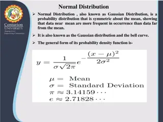
Normal distribution is a continuous probability
distribution which is bell shaped, unimodal and
symmetrical.
It is also known as Gaussian distribution
.
The
Normal
Distribution:
Definition
of
Terms
and
Symbols
Used
Characteristics
of
Normal
Distribution:
1)
It
is
“Bell-Shaped”
and
has
a
single
peak
at
the
center
of
the
distribution,
2)
The
arithmetic
Mean,
Median
and
Mode
are
equal.
3)
The
total
area
under
the
curve
is
1.00; half
the
area
under
the
normal
curve
is
to
the
right
of
this
center
point
and
the
other
half
to
the
left of
it,
4)
It
is
Symmetrical
about
the
mean,
5)
It
is
Asymptotic:
The
curve
gets
closer
and
closer
to
the
X
–
axis
but
never
actually touches
it.
To
put
it another
way,
the
tails
of
the
curve
extend
indefinitely
in
both
directions.
6)
The
location
of
a
normal
distribution
is
determined
by
the
Mean,
µ
,
the
Dispersion or
spread
of
the
distribution
is
determined
by
the Standard
Deviation,
σ
.
The
Normal
Distribution:
Graphically
Normal
Curve
is
Symmetrical
Two
halves
identical
Mean,
Median
and
Mode are
equal.
Theoretically,
curve
extends
to
-
∞
Theoretically,
curve
extends
to
+
∞
Many things closely follow a Normal Distribution:
•
heights of people
•
size of things produced by machines
•
errors in measurements
•
blood pressure
•
marks on a test
What is Uniform Distribution?
•
In statistics, uniform distribution is a term used to describe
a form of probability distribution where every possible
outcome has an equal likelihood of happening. The
probability is constant since each variable has equal
chances of being the outcome.
•
A deck of cards has within it uniform distributions
because the likelihood of drawing a heart, a club, a
diamond or a spade is equally likely. A coin also has a
uniform distribution because the probability of getting
either heads or tails in a coin toss is the same.
•
The uniform distribution can be visualized as a straight
horizontal line, so for a coin flip returning a head or tail,
both have a probability p = 0.50
Types of Uniform Distribution
Uniform distribution can be grouped into two categories based on the
types of possible outcomes.
1.
Discrete uniform distribution
2.
Continuous uniform distribution
Discrete uniform distribution
In statistics and probability theory, a discrete uniform distribution is a
statistical distribution where the probability of outcomes is equally likely
and with finite values. A good example of a discrete uniform distribution
would be the possible outcomes of rolling a fair 6-sided die. The possible
values would be 1, 2, 3, 4, 5, or 6. In this case, each of the six numbers
has an equal chance of appearing. Therefore, each time the 6-sided die is
thrown, each side has a chance of 1/6.
The number of values is finite. It is impossible to get a value of 1.3, 4.2,
or 5.7 when rolling a fair die.
However, if another die is added and they are both thrown, the
distribution that results is no longer uniform because the probability of
the sums is not equal.
Another simple example is the probability distribution of a coin being
flipped. The possible outcomes in such a scenario can only be two.
Therefore, the finite value is 2.
Continuous uniform distribution
Not all uniform distributions are discrete; some are
continuous. A continuous uniform distribution (also referred to
as rectangular distribution) is a statistical distribution with an
infinite number of equally likely measurable values.
A continuous uniform distribution usually comes in a
rectangular shape. A good example of a continuous uniform
distribution is an idealized
random number generator
. With
continuous uniform distribution, just like discrete uniform
distribution, every variable has an equal chance of happening.
However, there is an infinite number of points that can exist
What is a Skewed Distribution?
It is the degree of distortion from the symmetrical bell curve or the normal distribution. It
measures the lack of symmetry in data distribution.
It differentiates extreme values in one versus the other tail. A symmetrical distribution will have
a skewness of 0.
If one tail is longer than another, the distribution is skewed. These distributions are sometimes
called asymmetric or asymmetrical distributions as they don’t show any kind of symmetry.
Symmetry means that one half of the distribution is a mirror image of the other half. For
example, the normal distribution is a symmetric distribution with no skew. The tails are exactly
the same.
A normal curve
A left-skewed distribution
has a long left tail. Left-skewed
distributions are also called negatively-skewed distributions.
That’s because there is a long tail in the negative direction on
the number line. The mean is also to the left of the peak.
A right-skewed distribution
has a long right tail. Right-skewed
distributions are also called positive-skew distributions. That’s
because there is a long tail in the positive direction on the
number line. The mean is also to the right of the peak
Mean and Median in Skewed Distributions
In a normal distribution, the mean and the median are the same number
while the mean and median in a skewed distribution become different
numbers:
A left-skewed, negative distribution will have the mean to the left of the
median or the mean is to the left of the peak
A right-skewed distribution will have the mean to the right of the
median.
Bimodal Distribution
The “bi” in bimodal distribution refers to “two” and modal refers to the
peaks. It can seem a little confusing because in statistics, the term
“mode” refers to the most common number. However, if you think about
it, the peaks in any distribution are the most common number(s). The two
peaks in a bimodal distribution also represent two local maximums; these
are points where the data points stop increasing and start decreasing.
Example of a Bimodal Data Set
To help to make sense of this definition, we will look at an example of a set with one
mode, and then contrast this with a bimodal data set. Suppose we have the following set
of data:
1, 1, 1, 2, 2, 2, 2, 3, 4, 5, 5, 6, 6, 6, 7, 7, 7, 8, 10, 10
We count the frequency of each number in the set of data:
1 occurs in the set three times
2 occurs in the set four times
3 occurs in the set one time
4 occurs in the set one time
5 occurs in the set two times
6 occurs in the set three times
7 occurs in the set three times
8 occurs in the set one time
9 occurs in the set zero times
10 occurs in the set two times
Here we see that 2 occurs most often, and so it is the mode of the data set.
We count the frequency of each number in the set of data:
1 occurs in the set three times
2 occurs in the set four times
3 occurs in the set one time
4 occurs in the set one time
5 occurs in the set two times
6 occurs in the set three times
7 occurs in the set five times
8 occurs in the set one time
9 occurs in the set zero times
10 occurs in the set five times
Here 7 and 10 occur five times. This is higher than any of the other data values. Thus we say that
the data set is bimodal, meaning that it has two modes. Any example of a bimodal dataset will
be similar to this.
non-symmetric bimodal
Here is an example. A medium size neighborhood 24-hour convenience store collected data
from 537 customers on the amount of money spent in a single visit to the store. The following
histogram displays the data.
Note that the overall shape of the distribution is skewed to the right with a clear mode around
$25. In addition, it has another (smaller) “peak” (mode) around $50-55.
The majority of the customers spend around $25 but there is a cluster of customers who enter
the store and spend around $50-55.
Spread
The spread of a distribution refers to the variability of the data. If the observations cover a wide
range, the spread is larger. If the observations are clustered around a single value, the spread is
smaller.
Outliers. Sometimes, distributions are characterized by extreme values that differ greatly from
the other observations. These extreme values are called outliers.
Kurtosis
Kurtosis is all about the tails of the distribution . It is used to describe the extreme values in one
versus the other tail. It is actually the measure of outliers present in the distribution.
High kurtosis in a data set is an indicator that data has heavy tails or outliers. If there is a high
kurtosis, then, we need to investigate why do we have so many outliers. It indicates a lot of
things, maybe wrong data entry or other things. Investigate!
Low kurtosis in a data set is an indicator that data has light tails or lack of outliers. If we get low
kurtosis(too good to be true), then also we need to investigate and trim the dataset of
unwanted results.
Types
Mesokurtic:
This distribution has kurtosis statistic similar to that of the normal distribution. It
means that the extreme values of the distribution are similar to that of a normal distribution
characteristic. This definition is used so that the standard normal distribution has a kurtosis of
three
Leptokurtic (Kurtosis > 3):
Distribution is longer, tails are fatter. Peak is higher and sharper than
Mesokurtic, which means that data are heavy-tailed or profusion of outliers.
Outliers stretch the horizontal axis of the histogram graph, which makes the bulk of the data
appear in a narrow (“skinny”) vertical range, thereby giving the “skinniness” of a leptokurtic
distribution.
Platykurtic: (Kurtosis < 3):
Distribution is shorter, tails are thinner than the normal distribution.
The peak is lower and broader than Mesokurtic, which means that data are light-tailed or lack of
outliers.
The reason for this is because the extreme values are less than that of the normal distribution.
Skewness vs. kurtosis
Skewness is a measure of symmetry, or more precisely, the lack of symmetry. A distribution, or
data set, is symmetric if it looks the same to the left and right of the center point. Kurtosis is a
measure of whether the data are heavy-tailed or light-tailed relative to a normal distribution.
A data distribution represents values and frequencies in ordered data. The normal distribution is bell-shaped, symmetrical, and represents probabilities in a continuous manner. It's characterized by features like a single peak, symmetry around the mean, and standard deviation. The uniform distribution, on the other hand, assigns equal probabilities to all possible outcomes. Both distributions have significant applications in various fields, and understanding them is crucial in statistical analysis.

Download Presentation

Please find below an Image/Link to download the presentation.
The content on the website is provided AS IS for your information and personal use only. It may not be sold, licensed, or shared on other websites without obtaining consent from the author. Download presentation by click this link. If you encounter any issues during the download, it is possible that the publisher has removed the file from their server.
E N D
Presentation Transcript
A data distribution is a function which shows all the possible values (or intervals) of the data. It also tells you how often each value occurs. Often, the data in a distribution will be ordered from smallest to largest, and graphs and charts allow you to easily see both the values and the frequency with which they appear. A distribution is simply a collection of data, or scores, on a variable. Usually, these scores are arranged in order from smallest to largest and then they can be presented graphically.
The Normal Distribution Normal distribution is a continuous probability distribution which is bell shaped, unimodal and symmetrical. It is also known as Gaussian distribution .
The Normal Distribution: Definition of Terms and Symbols Used Characteristics of Normal Distribution: It is Bell-Shaped and has a single peak at the center of the distribution, 2) ThearithmeticMean, Medianand Modeareequal. The total area under the curve is 1.00; half the area under the normal curve is to the right of this center point and the other half to the leftofit, 4) Itis Symmetrical aboutthemean, It is Asymptotic: The curve gets closer and closer to the X axis but never actually touches it. To put it another way, the tailsof thecurveextend indefinitelyin bothdirections. 6) Thelocationof anormaldistributionisdetermined bythe Mean, , the Dispersion or spread of the distribution is determined by the Standard Deviation, . 1) 3) 5)
The Normal Distribution:Graphically Normal Curve isSymmetrical Two halvesidentical Theoretically,curve extends to - Theoretically,curve extends to + Mean, Median and Mode are equal.
Many things closely follow a Normal Distribution: heights of people size of things produced by machines errors in measurements blood pressure marks on a test
What is Uniform Distribution? In statistics, uniform distribution is a term used to describe a form of probability distribution where every possible outcome has an equal likelihood of happening. The probability is constant since each variable has equal chances of being the outcome. A deck of cards has within it uniform distributions because the likelihood of drawing a heart, a club, a diamond or a spade is equally likely. A coin also has a uniform distribution because the probability of getting either heads or tails in a coin toss is the same. The uniform distribution can be visualized as a straight horizontal line, so for a coin flip returning a head or tail, both have a probability p = 0.50
Types of Uniform Distribution Uniform distribution can be grouped into two categories based on the types of possible outcomes. 1. Discrete uniform distribution 2. Continuous uniform distribution Discrete uniform distribution In statistics and probability theory, a discrete uniform distribution is a statistical distribution where the probability of outcomes is equally likely and with finite values. A good example of a discrete uniform distribution would be the possible outcomes of rolling a fair 6-sided die. The possible values would be 1, 2, 3, 4, 5, or 6. In this case, each of the six numbers has an equal chance of appearing. Therefore, each time the 6-sided die is thrown, each side has a chance of 1/6.
The number of values is finite. It is impossible to get a value of 1.3, 4.2, or 5.7 when rolling a fair die. However, if another die is added and they are both thrown, the distribution that results is no longer uniform because the probability of the sums is not equal. Another simple example is the probability distribution of a coin being flipped. The possible outcomes in such a scenario can only be two. Therefore, the finite value is 2.
Continuous uniform distribution Not all uniform distributions are discrete; some are continuous. A continuous uniform distribution (also referred to as rectangular distribution) is a statistical distribution with an infinite number of equally likely measurable values. A continuous uniform distribution usually comes in a rectangular shape. A good example of a continuous uniform distribution is an idealized random number generator. With continuous uniform distribution, just like discrete uniform distribution, every variable has an equal chance of happening. However, there is an infinite number of points that can exist
What is a Skewed Distribution? It is the degree of distortion from the symmetrical bell curve or the normal distribution. It measures the lack of symmetry in data distribution. It differentiates extreme values in one versus the other tail. A symmetrical distribution will have a skewness of 0. If one tail is longer than another, the distribution is skewed. These distributions are sometimes called asymmetric or asymmetrical distributions as they don t show any kind of symmetry. Symmetry means that one half of the distribution is a mirror image of the other half. For example, the normal distribution is a symmetric distribution with no skew. The tails are exactly the same. A normal curve
A left-skewed distribution has a long left tail. Left-skewed distributions are also called negatively-skewed distributions. That s because there is a long tail in the negative direction on the number line. The mean is also to the left of the peak. A right-skewed distribution has a long right tail. Right-skewed distributions are also called positive-skew distributions. That s because there is a long tail in the positive direction on the number line. The mean is also to the right of the peak
Mean and Median in Skewed Distributions In a normal distribution, the mean and the median are the same number while the mean and median in a skewed distribution become different numbers: A left-skewed, negative distribution will have the mean to the left of the median or the mean is to the left of the peak A right-skewed distribution will have the mean to the right of the median.
Bimodal Distribution The bi in bimodal distribution refers to two and modal refers to the peaks. It can seem a little confusing because in statistics, the term mode refers to the most common number. However, if you think about it, the peaks in any distribution are the most common number(s). The two peaks in a bimodal distribution also represent two local maximums; these are points where the data points stop increasing and start decreasing.
Example of a Bimodal Data Set To help to make sense of this definition, we will look at an example of a set with one mode, and then contrast this with a bimodal data set. Suppose we have the following set of data: 1, 1, 1, 2, 2, 2, 2, 3, 4, 5, 5, 6, 6, 6, 7, 7, 7, 8, 10, 10 We count the frequency of each number in the set of data: 1 occurs in the set three times 2 occurs in the set four times 3 occurs in the set one time 4 occurs in the set one time 5 occurs in the set two times 6 occurs in the set three times 7 occurs in the set three times 8 occurs in the set one time 9 occurs in the set zero times 10 occurs in the set two times Here we see that 2 occurs most often, and so it is the mode of the data set.
We count the frequency of each number in the set of data: 1 occurs in the set three times 2 occurs in the set four times 3 occurs in the set one time 4 occurs in the set one time 5 occurs in the set two times 6 occurs in the set three times 7 occurs in the set five times 8 occurs in the set one time 9 occurs in the set zero times 10 occurs in the set five times Here 7 and 10 occur five times. This is higher than any of the other data values. Thus we say that the data set is bimodal, meaning that it has two modes. Any example of a bimodal dataset will be similar to this.
non-symmetric bimodal Here is an example. A medium size neighborhood 24-hour convenience store collected data from 537 customers on the amount of money spent in a single visit to the store. The following histogram displays the data. Note that the overall shape of the distribution is skewed to the right with a clear mode around $25. In addition, it has another (smaller) peak (mode) around $50-55. The majority of the customers spend around $25 but there is a cluster of customers who enter the store and spend around $50-55.
Spread The spread of a distribution refers to the variability of the data. If the observations cover a wide range, the spread is larger. If the observations are clustered around a single value, the spread is smaller.
Outliers. Sometimes, distributions are characterized by extreme values that differ greatly from the other observations. These extreme values are called outliers.
Kurtosis Kurtosis is all about the tails of the distribution . It is used to describe the extreme values in one versus the other tail. It is actually the measure of outliers present in the distribution. High kurtosis in a data set is an indicator that data has heavy tails or outliers. If there is a high kurtosis, then, we need to investigate why do we have so many outliers. It indicates a lot of things, maybe wrong data entry or other things. Investigate! Low kurtosis in a data set is an indicator that data has light tails or lack of outliers. If we get low kurtosis(too good to be true), then also we need to investigate and trim the dataset of unwanted results. Types Mesokurtic: This distribution has kurtosis statistic similar to that of the normal distribution. It means that the extreme values of the distribution are similar to that of a normal distribution characteristic. This definition is used so that the standard normal distribution has a kurtosis of three
Leptokurtic (Kurtosis > 3): Distribution is longer, tails are fatter. Peak is higher and sharper than Mesokurtic, which means that data are heavy-tailed or profusion of outliers. Outliers stretch the horizontal axis of the histogram graph, which makes the bulk of the data appear in a narrow ( skinny ) vertical range, thereby giving the skinniness of a leptokurtic distribution. Platykurtic: (Kurtosis < 3): Distribution is shorter, tails are thinner than the normal distribution. The peak is lower and broader than Mesokurtic, which means that data are light-tailed or lack of outliers. The reason for this is because the extreme values are less than that of the normal distribution.
Skewness vs. kurtosis Skewness is a measure of symmetry, or more precisely, the lack of symmetry. A distribution, or data set, is symmetric if it looks the same to the left and right of the center point. Kurtosis is a measure of whether the data are heavy-tailed or light-tailed relative to a normal distribution.


: Distribution is longer, tails")