Understanding Multinomial Distribution in Statistical Analysis


Multinomial Distribution
World Premier League Soccer Game
Outcomes

Multinomial Distribution
•
Used to model a series of
n
independent trials, where each
trial has
k
possible outcomes (categories)
•
The probability of
i
th
category occurring on any given trial is
p
i
subject to
p
1
+
p
2
+ … +
p
k
= 1
•
The random variable
Y
i
denotes the number of trials in
which the
i
th
category occurred:
Y
1
+
Y
2
+ … +
Y
k
=
n
•
Note that once we have observed
Y
1
,
Y
2
, …,
Y
k-1
, we have
Y
k
=
n
-
Y
1
- … -
Y
k-1
similarly,
p
k
= 1 -
p
1
- … -
p
k-1
Multinomial Distribution – Mathematical Form - I
Multinomial Distribution – Mathematical Form - II
Multinomial Distribution – Mathematical Form - III
Examples – World Premier Soccer Leagues
•
Nations: England, France, Germany, Italy, Spain (2013)
•
League Play: Each team plays all remaining teams twice
(once Home, once Away)
•
Games can end in one of 3 possible ways with respect to
Home Team: Win, Draw (Tie), Lose
Probability Calculations
Distribution of Number of Points in Sample
Points are assigned such that a Win gets 3 Points, Draw gets 1, Loss gets 0
Multinomial Distribution is a powerful tool used in statistical analysis to model outcomes of events with multiple categories. This distribution is applied to scenarios where each trial has several possible outcomes, and the sum of probabilities of all outcomes is equal to 1. By defining random variables and exploring mathematical forms, Multinomial Distribution helps analyze and predict outcomes in various fields, including the World Premier League Soccer game outcomes. The expansion, moment generating function, and alternative approaches for obtaining covariances provide a comprehensive understanding of this distribution.

Download Presentation

Please find below an Image/Link to download the presentation.
The content on the website is provided AS IS for your information and personal use only. It may not be sold, licensed, or shared on other websites without obtaining consent from the author. Download presentation by click this link. If you encounter any issues during the download, it is possible that the publisher has removed the file from their server.
E N D
Presentation Transcript
Multinomial Distribution World Premier League Soccer Game Outcomes
Multinomial Distribution Used to model a series of n independent trials, where each trial has k possible outcomes (categories) The probability of ithcategory occurring on any given trial is pisubject to p1+ p2+ + pk= 1 The random variable Yidenotes the number of trials in which the ithcategory occurred: Y1+ Y2+ + Yk= n Note that once we have observed Y1, Y2, , Yk-1, we have Yk= n - Y1- - Yk-1 similarly, pk= 1 - p1- - pk-1
Multinomial Distribution Mathematical Form - I n = ! !... k n ( ) ( ) n + + + = m k m m Multinomial Expansion: ... ... a a a a a a a k 1 2 1 2 1 2 i k ! ! m m m = + + + = 1 ... i m m m n 1 2 k 1 2 k ( ) ( ) = = = = = In terms of the RVs: ,..., : , ,..., , ,... Y Y P Y y Y y Y y p y y y 1 1 1 1 2 2 1 1 1 2 1 k k k k ! n ( ) n y ... y y = y k y y ... 1 ... p p p p p p 1 2 1 k 1 1 2 k ( ) 1 2 1 1 2 1 k ! !... ! .. . ! y y y n y y y 1 2 1 1 2 1 k k + + + = Note that these probabilities sum to 1 over all possible outcomes where ... y y y n 1 2 k = ( n ) + + = ... 1 1 t Y t Y Moment Generating Function: , ..., m t t t E e 1 1 k k 1 ! 2 1 k ( ) n y ... y y + + = = ... 1 1 t y t y y k y y ... 1 ... e p p p p p p 1 2 1 k 1 1 1 k k k 1 2 ( ) 1 2 1 1 2 1 k ! !... ! ... ! y y y n y y y 1 2 1 1 2 1 k k ! y n ( ) ( ) ( ) y n y = + + + t y k t 1 t t k 1 ... ... p e p e p p e p e p 1 1 k k k 1 1 1 1 1 1 k k k ! !... ! ! y y y 1 2 1 k k Marginal Distribu ( 1 ,0,....0 m t tion of obtained by evaluating Y 1 ) ( = ) ( ) n n ( ) ( ) + + + + = + = t t ... 1 ~ , 1,..., p e p p p p e p Y Bin n p i k 1 1 1 2 1 1 1 k k i i
Multinomial Distribution Mathematical Form - II Marginal Distribution of obtained by evaluating Y 1 ) ( np = ) ( ) n n ( ( ) ( ) = + + + + = + = t t ,0,....0 ... 1 ~ , 1,..., m t p e p p p p e p Y Bin n p i k 1 1 1 1 2 1 1 1 k k i i E Y ( ) = 1 V Y np p i i i i i Alternative Approach (also used to obtain Covariances): 1 if i U = 0 otherwise = + = Trial is in Category i 1 if Trial is in Category ' 0 otherwise + j i j = W i ( ) ( ) ( ) ( ) E U = = 2 i 2 2 1 0 1 1 0 1 p p p E U p p p i j j j j j j V U ( ) ( ) ( ) 2 E W V W = = = = 1 1 p p p p p p p ' ' ' j j j j j i j i j j V Y = = = Trials are independent , , , 0 ' COV U U COV U W COV W W i i ' ' ' i i i i i i n E Y ( ) = = = 1 Y U np np p j i j j j j j = 1 i n E Y V Y ( ) = = = 1 Y W np np p ' ' ' ' ' ' j i j j j j j = 1 i
Multinomial Distribution Mathematical Form - III i Obtaining , ': COV Y Y j j ' j j 1 if Trial is in Category 0 otherwise 1 if Trial is in Category ' 0 otherwise j i j = = U W i i = = Note: 0 since , i only 1 category can occur on each trial 0 UW E UW i i i i i E U = = = 0 COV U W E UW E W p p p p ' ' i i i i j j j j Trials are independent , i COV U U = = = , , 0 ' COV U W COV W W i i ' ' ' i i i i i n n n n ) = = + = , , , , COV Y Y COV U W COV U W COV U W ' ' j j i i i i i i = = = = 1 1 1 1 ' i i i i i i ( = = n p p np p ' ' j j j j
Examples World Premier Soccer Leagues Nations: England, France, Germany, Italy, Spain (2013) League Play: Each team plays all remaining teams twice (once Home, once Away) Games can end in one of 3 possible ways with respect to Home Team: Win, Draw (Tie), Lose Win (1) p1 0.4711 0.4395 0.4739 0.4763 0.4711 Draw (2) p2 0.2053 0.2868 0.2092 0.2368 0.2263 Lose (3) p3 0.3237 0.2737 0.3170 0.2868 0.3026 League England France Germany Italy Spain
Probability Calculations All calculations based on assumption of their being an infinite population of games Sample 8 Games from each league, probability of: 4 Wins, 2 Draws, 2 Losses: 4, 2, 2 4,2,2 8! England: 4,2,2 4! ( ) ( ) ( France: 4,2,2 .4395 .2868 4!2!2! 8! Germany: 4,2,2 .4739 .2092 4!2!2! 8! Italy: 4,2,2 .4763 .2368 4!2!2! 8! Spain: 4,2,2 .4711 .22 4!2!2! ( ) ( ) = = = = P Y Y Y p 1 2 3 ( ) ( ) ( ) ( ) 4 2 2 = = .4711 .2053 .3237 .0914 p 2!2! 8! ) ( ) 4 2 2 = = .2737 .0966 p ( ) ( ) ( ) ( ) 4 2 2 = = .3170 .0932 p ( ) ( ) ( ) ( ) 4 2 2 = = .2868 .0997 p ( ) ( ) ( ) ( ) 4 2 2 = = 63 .3026 .0970 p
Distribution of Number of Points in Sample Points are assigned such that a Win gets 3 Points, Draw gets 1, Loss gets 0 = + + = + 3 1 0 3 1 P Y Y Y Y Y 1 2 3 1 2 E P E Y E Y = + = + 3 3 np np 1 2 1 2 V Y ( )( ) 2 3 1 ( ) ( ) ( ) = + + = + + 2 2 3 1 , 9 1 1 6 V P V Y COV Y Y np p np p np p 1 2 1 2 1 1 2 2 1 2 E P ( ) ( ) = = + = + 8 24 8 72 1 8 1 48 n p p V P p p p p p p 1 2 1 1 2 2 1 2 E P E P ( ( ( ( ( ) ) ) ) ) ( ( ( ( ( ) ) ) ) ) V P = = = = = + + + + + = = = = = = = = = = = = = = = England: 24 .4711 8 .2053 12.95 14.60 3.82 E P V P P France: 24 . 4395 8 .2868 12.84 13.32 3.65 V P P Germany: 24 .4739 8 .2092 13.05 14.52 3.81 E P V P P Italy: 24 .4763 8 .2368 13.33 13.99 3.74 E P V P P Spain: 24 .4711 8 .2263 13.12 14.22 3.77 P