Introduction to Data Analysis in Geophysics using MATLAB Graphics Handles
Practice interactive input, file reading, and plotting in MATLAB Graphics Handles lab. Explore ways to improve graphics in Geophysics data analysis. Learn basic histogram plot representation with properties and understand the functionalities provided in MATLAB for handling geophysical data through graphical visualization. Discover advanced techniques to enhance graphics through interactive elements and file manipulation.

Download Presentation

Please find below an Image/Link to download the presentation.
The content on the website is provided AS IS for your information and personal use only. It may not be sold, licensed, or shared on other websites without obtaining consent from the author. Download presentation by click this link. If you encounter any issues during the download, it is possible that the publisher has removed the file from their server.
E N D
Presentation Transcript
C E R I C E R I- -7 1 04/ C IV L 7 1 04/ C IV L - -8 1 2 6 D ata A nalysis in G eophysics 8 1 2 6 D ata A nalysis in G eophysics C ontinue Introduction to M atlab G raphics H andles L ab: practice with interactive input, reading file, and plotting. L ab 9 , 09 / 2 4/ 1 9
M ore on G raphics H andles H ow to improve the graphics. S ee how2handlegraphics.m
>> get(0) CallbackObject: [0 0 GraphicsPlaceholder] Children: [1 1 Figure] CurrentFigure: [1 1 Figure] FixedWidthFontName: 'Courier New' HandleVisibility: 'on' MonitorPositions: [1 1 1440 900] Parent: [0 0 GraphicsPlaceholder] PointerLocation: [219 68] ScreenDepth: 32 ScreenPixelsPerInch: 72 ScreenSize: [1 1 1440 900] ShowHiddenHandles: 'off' Tag: '' Type: 'root' Units: 'pixels' UserData: [] >> get(0,'default') ans = struct with fields: defaultFigurePosition: [440 378 560 420] defaultFigurePaperPositionMode: 'auto' defaultAxesColorOrder: [0 0 0] defaultAxesLineStyleOrder: [5 2 char] defaultAxesFontSize: 18 defaultTextFontSize: 16 defaultLineLineWidth: 3 >>
>> a=gcf a = Figure (1: basic histogram plot) with properties: Number: 1 Name: 'basic histogram plot' Color: [0.940000000000000 0.940000000000000 0.940000000000000] Position: [440 378 560 420] Units: 'pixels' Show all properties >> gcf gets current figure handle. N ext slide shows what happens when you click on show all properties
Show all properties Alphamap: [1 64 double] BeingDeleted: 'off' BusyAction: 'queue' ButtonDownFcn: '' Children: [1 1 Axes] Clipping: 'on' CloseRequestFcn: 'closereq' Color: [0.940000000000000 0.940000000000000 0.940000000000000] Colormap: [64 3 double] CreateFcn: '' CurrentAxes: [1 1 Axes] CurrentCharacter: ')' CurrentObject: [0 0 GraphicsPlaceholder] CurrentPoint: [0 0] DeleteFcn: '' DockControls: 'on' FileName: '' GraphicsSmoothing: 'on' HandleVisibility: 'on' InnerPosition: [440 378 560 420] IntegerHandle: 'on' Interruptible: 'on' InvertHardcopy: 'on' KeyPressFcn: '' KeyReleaseFcn: '' MenuBar: 'figure' Name: 'basic histogram plot' NextPlot: 'add' Number: 1 NumberTitle: 'on' OuterPosition: [440 378 560 493] PaperOrientation: 'portrait' PaperPosition: [0.361111111111111 2.583333333333334 7.777777777777779 5.833333333333332] PaperPositionMode: 'auto' PaperSize: [8.500000000000000 11] PaperType: 'usletter' PaperUnits: 'inches' Parent: [1 1 Root] Pointer: 'arrow' PointerShapeCData: [16 16 double] PointerShapeHotSpot: [1 1] Position: [440 378 560 420] Renderer: 'opengl' RendererMode: 'auto' Resize: 'on' Scrollable: 'off' SelectionType: 'normal' SizeChangedFcn: '' Tag: '' ToolBar: 'auto' Type: 'figure' UIContextMenu: [0 0 GraphicsPlaceholder] Units: 'pixels' UserData: [] Visible: 'on' WindowButtonDownFcn: '' WindowButtonMotionFcn: '' WindowButtonUpFcn: '' WindowKeyPressFcn: '' WindowKeyReleaseFcn: '' WindowScrollWheelFcn: '' WindowState: 'normal' WindowStyle: 'normal' XDisplay: 'Quartz
>> c=gca c = Axes (basic histogram plot) with properties: XLim: [-3.300000000000000 3.300000000000000] YLim: [0 400] XScale: 'linear' YScale: 'linear' GridLineStyle: '-' Position: [0.130000000000000 0.123333333333333 0.775000000000000 0.801666666666667] Units: 'normalized' Show all properties >> N ext slide shows what happens when you click on show all properties (there are 1 3 8 things in the list!!)
Show all properties ALim: [0 1] ALimMode: 'auto' ActivePositionProperty: 'outerposition' AlphaScale: 'linear' Alphamap: [1 64 double] AmbientLightColor: [1 1 1] BeingDeleted: 'off' Box: 'on' BoxStyle: 'back' BusyAction: 'queue' ButtonDownFcn: '' CLim: [0 1] CLimMode: 'auto' CameraPosition: [0 200 17.320508075688771] CameraPositionMode: 'auto' CameraTarget: [0 200 0] CameraTargetMode: 'auto' CameraUpVector: [0 1 0] CameraUpVectorMode: 'auto' CameraViewAngle: 6.608610360311924 CameraViewAngleMode: 'auto' Children: [1 1 Histogram] Clipping: 'on' ClippingStyle: '3dbox' Color: [1 1 1] ColorOrder: [0 0 0] ColorOrderIndex: 1 ColorScale: 'linear' Colormap: [64 3 double] CreateFcn: '' CurrentPoint: [2 3 double] DataAspectRatio: [3.300000000000000 200 1] DataAspectRatioMode: 'auto' DeleteFcn: '' FontAngle: 'normal' FontName: 'Helvetica' FontSize: 18 FontSizeMode: 'auto' FontSmoothing: 'on' FontUnits: 'points' FontWeight: 'normal' GridAlpha: 0.150000000000000 GridAlphaMode: 'auto' GridColor: [0.150000000000000 0.150000000000000 0.150000000000000] GridColorMode: 'auto' GridLineStyle: '-' HandleVisibility: 'on' HitTest: 'on' Interactions: [1 1 matlab.graphics.interaction.interface.DefaultAxesInteractionSet] Interruptible: 'on' LabelFontSizeMultiplier: 1.100000000000000 Layer: 'bottom' Legend: [0 0 GraphicsPlaceholder] LineStyleOrder: [5 2 char] LineStyleOrderIndex: 1
T his web page has the documentation for all the graphics object properties https://www.mathworks.com/help/matla b/graphics-object-properties.html G o there to see how it is organized.
A nother example of tex and the gibberish you have to type/ understand to make pretty output (T E K is a typesetting program and makes the prettiest outputs but at a cost! Y ou can guess how it works reading it and looking at the output, but it is hard to come up with it.) \[ \int_a^bu\frac{d^2v}{dx^2}\,dx =\left.u\frac{dv}{dx}\right|_a^b -\int_a^b\frac{du}{dx}\frac{dv}{dx}\,dx. \]
A nd another Typesetting continued fractions is easy: \[ x = a_0 + \frac{1}{a_1 + \frac{1}{a_2 + \frac{1}{a_3 + a_4}}} \] T his is pretty much the antithesis of the W Y S IW Y G W W hat Y Y ou G G et ) philosophy of M S W ord, P ages (A pples version of W ord). etc. W Y S IW Y G (an acronym for W W hat Y Y ou S S ee IIs
H ow turn off underscore signifying next character is a subscript (default intrepreter is T E X ). T his way you don t have to escape the underscore ( \_ ) to get it to be an underscore. T his is needed when the text is not hard coded , eg. a file name. S et the Interpreter property for that field to 'none'; the default for text() fields is T E X . title('This_title has an underline', 'Interpreter', 'none');
W rite script to read the files mixedin1.dat and mixedin2.dat T hese files have earthquake data. M ost earthquake data files have a mixture of numbers and text (the first file) and time formatted data, and a header (that typically identifies the data columns (the second file).
Prompt for file name Empty response? File exists? Read file into inbuf Display line Prompt for positions in input line of x and y data to plot Get number lines Preallocate memory (for speed, need to know how many lines in input file) Loop over lines to pull (x,y) data out of input cell array Plot x,y data
A nother way to read data a line at a time fgets and fgetl. F irst one keeps newline character, second one drops the newline character see red stuff below >> tline = fgets(fid) tline = '2014 04 26 -55.8259 -27.1533 34.93 4.6 2014-04-26T02:02:20.930Z near s georgia tline = fgetl(fid) tline = '2014 04 01 -60.1681 -24.8498 10 4.9 2014-04-01T08:29:13.300 near s georgia A s you read the file a line at at time it advances through the file. If need to go back to the beginning you have to rewind. frewind(fid)
Y ou can also give handles to functions, this allows you to pass functions as arguments to other functions f = @(x) x.^3 -3*x+1; T hen call f(3.4) etc., (like sin, cosine, etc.) T his also makes function handles so you can pass functions to other functions X=linspace(0,2); Plot(x,f(x))


")