MATLAB Basics for Electrical Engineering Students

In this instructional content from the Government Polytechnic West Champaran Department of Electrical Engineering, students are introduced to the fundamentals of MATLAB. Topics covered include transposing matrices, concatenating matrices, matrix generators, arrays, entering matrices, and manipulating vectors. The content explains the basics of matrices in MATLAB, creating column and row vectors, accessing elements in vectors, using colon notation for element selection, and entering matrices into MATLAB.

Download Presentation

Please find below an Image/Link to download the presentation.
The content on the website is provided AS IS for your information and personal use only. It may not be sold, licensed, or shared on other websites without obtaining consent from the author. Download presentation by click this link. If you encounter any issues during the download, it is possible that the publisher has removed the file from their server.
E N D
Presentation Transcript
Government Polytechnic west Champaran Department : Electrical Engineering MATLAB subject code: 2020409
Content 1. 2. 3. 4. 5. 6. 7. 8. 9. 10. Transposing a matrix 11. Concatenating matrices 12. Matrix generators Arrays & Matrices Entering a matrix Matrix indexing Colon operator Linear spacing Colon operator in a matrix Creating a sub-matrix Deleting row or column Dimension
Arrays & Matrices Matrices are the basic elements of the MATLAB environment. A matrix is a two- dimensional array consisting of m rows and n columns. Special cases are column vectors (n = 1) and row vectors (m = 1). Entering a vector >> v = [1 4 7 10 13] v = 1 4 7 10 13 Column vectors are created in a similar way, however, semicolon (;) must separate the components of a column vector >> w = [1;4;7;10;13]
Continuation w = 1 4 7 10 13 On the other hand, a row vector is converted to a column vector using the transpose operator. The transpose operation is denoted by an apostrophe or a single quote ( ).
Continuation >> w = v w = 1 4 7 10 13 Thus, v(1) is the first element of vector v, v(2) its second element, and so forth.
Continuation to access blocks of elements, we use MATLAB s colon notation (:). For example, to access the first three elements of v, we write, >> v(1:3) ans = 1 4 7 Or, all elements from the third through the last elements, >> v(3:end) ans = 7 10 13
Continuation where end signifies the last element in the vector. If v is a vector, writing >> v(:) produces a column vector, where as writing >> v(1:end) produces a row vector.
Entering a matrix A matrix is an array of numbers. To type a matrix into MATLAB you must begin with a square bracket, [ separate elements in a row with spaces or commas (,) use a semicolon (;) to separate rows end the matrix with another square bracket, ]. >> A = [1 2 3; 4 5 6; 7 8 9]
Continuation MATLAB then displays the 3 3 matrix as follows, A = 1 2 3 4 5 6 7 8 9 Note that the use of semicolons (;) here is different from their use mentioned earlier to suppress output or to write multiple commands in a single line.
Continuation We can then view a particular element in a matrix by specifying its location. We write, >> A(2,1) ans = 4 A(2,1) is an element located in the second row and first column. Its value is 4.
Matrix indexing We select elements in a matrix just as we did for vectors, but now we need two indices. The element of row i and column j of the matrix A is denoted by A(i,j). Thus, A(i,j) in MATLAB refers to the element Aij of matrix A. The first index is the row number and the second index is the column number. For example, A(1,3) is an element of first row and third column. Here, A(1,3)=3. Correcting any entry is easy through indexing. Here we substitute A(3,3)=9 by A(3,3)=0.
Continuation >> A(3,3) = 0 A = 1 2 3 4 5 6 7 8 0 Single elements of a matrix are accessed as A(i,j), where i 1 and j 1. Zero or negative subscripts are not supported in MATLAB.
Colon operator The colon operator will prove very useful and understanding how it works is the key to efficient and convenient usage of MATLAB. It occurs in several different forms. Often we must deal with matrices or vectors that are too large to enter one element at a time. For example, suppose we want to enter a vector x consisting of points (0, 0.1, 0.2, 0.3, , 5). We can use the command >> x = 0:0.1:5; The row vector has 51 elements.
Linear spacing On the other hand, there is a command to generate linearly spaced vectors: linspace. It is similar to the colon operator (:), but gives direct control over the number of points. For example, y = linspace(a,b) generates a row vector y of 100 points linearly spaced between and including a and b. y = linspace(a,b,n) generates a row vector y of n points linearly spaced between and including a and b. This is useful when we want to divide an interval into a number of subintervals of the same length. For example
Continuation >> theta = linspace(0,2*pi,101) divides the interval [0, 2 ] into 100 equal subintervals, then creating a vector of 101 elements.
Colon operator in a matrix The colon operator can also be used to pick out a certain row or column. For example, the statement A(m:n,k:l specifies rows m to n and column k to l. Subscript expressions refer to portions of a matrix. For example, >> A(2,:) ans = 4 5 6 is the second row elements of A. The colon operator can also be used to extract a sub-matrix from a matrix A.
Continuation >> A(:,2:3) ans = 2 3 5 6 8 0 A(:,2:3) is a sub-matrix with the last two columns of A. A row or a column of a matrix can be deleted by setting it to a null vector, [ ]. >>A(:,2)=[] ans = 1 3 4 6 7 0
Creating a sub-matrix To extract a submatrix B consisting of rows 2 and 3 and columns 1 and 2 of the matrix A, do the following. >> B = A([2 3],[1 2]) B = 4 5 7 8 To interchange rows 1 and 2 of A, use the vector of row indices together with the colon operator.
Continuation >> C = A([2 1 3],:) C = 4 5 6 1 2 3 7 8 0 It is important to note that the colon operator (:) stands for all columns or all rows. To create a vector version of matrix A, do the following.
Continuation >> A(:) ans = 1 2 3 4 5 6 7 8 0
Continuation The submatrix comprising the intersection of rows p to q and columns r to s is denoted by A(p:q,r:s). As a special case, a colon (:) as the row or column specifier covers all entries in that row or column; thus A(:,j) is the jth column of A, while A(i,:) is the ith row, and A(end,:) picks out the last row of A. The keyword end, used in A(end,:), denotes the last index in the specified dimension. Here are some examples.
Continuation >> A >> A(end:-1:1,end) 1 2 3 ans = 4 5 6 9 7 8 9 6 >> A(2:3,2:3) 3 ans = >> A([1 3],[2 3]) 5 6 ans = 8 9 2 3 8 9
Deleting row or column To delete a row or column of a matrix, use the empty vector operator, [ ]. >> A(3,:) = [] A = 1 2 3 4 5 6 Third row of matrix A is now deleted. To restore the third row, we use a technique for creating a matrix.
Continuation >> A = [A(1,:);A(2,:);[7 8 0]] A = 1 2 3 4 5 6 7 8 0 Matrix A is now restored to its original form.
Dimension To determine the dimensions of a matrix or vector, use the command size. For example >> size(A) ans = 3 3 means 3 rows and 3 columns. Or more explicitly with, >> [m,n]=size(A)
Transposing a matrix The transpose operation is denoted by an apostrophe or a single quote ( ). It flips a matrix about its main diagonal and it turns a row vector into a column vector. Thus >> A ans = 1 4 7 2 5 8 3 6 0 By using linear algebra notation, the transpose of m n real matrix A is the n m matrix that results from interchanging the rows and columns of A. The transpose matrix is denoted ?? .
Concatenating matrices Matrices can be made up of sub-matrices. Here is an example. First, let s recall our previous matrix A. A = 1 2 3 4 5 6 7 8 9 The new matrix B will be, >> B = [A 10*A; -A [1 0 0; 0 1 0; 0 0 1]] B = 1 2 3 10 20 30
Continuation B = 1 2 3 10 20 30 4 5 6 40 50 60 7 8 9 70 80 90 -1 -2 -3 1 0 0 -4 -5 -6 0 1 0 -7 -8 -9 0 0 1
Matrix generators MATLAB provides functions that generates elementary matrices. The matrix of zeros, the matrix of ones, and the identity matrix are returned by the functions zeros, ones, and eye, respectively. Elementary matrices
Continuation For a complete list of elementary matrices and matrix manipulations, type help elmat or doc elmat. Here are some examples: 1. >> b=ones(3,1) 2. >> eye(3) b = ans = 1 1 0 0 1 0 1 0 1 0 0 1 Equivalently, we can define b as >> b=[1;1;1]
Continuation 3. >> c=zeros(2,3) c = 0 0 0 0 0 0 In addition, it is important to remember that the three elementary operations of addition (+), subtraction ( ), and multiplication ( ) apply also to matrices whenever the dimensions are compatible. Two other important matrix generation functions are rand and randn, which generate matrices of (pseudo-)random numbers using the same syntax as eye.
Continuation In addition, matrices can be constructed in a block form. With C defined by C = [1 2; 3 4], we may create a matrix D as follows >> D = [C zeros(2); ones(2) eye(2)] D = 1 2 0 0 3 4 0 0 1 1 1 0 1 1 0 1
Array operations and Linear equations Matrix arithmetic operations MATLAB allows arithmetic operations: +, , , and to be carried out on matrices. Thus, A+B or B+A is valid if A and B are of the same size A*B is valid if A s number of column equals B s number of rows A^2 is valid if A is square and equals A*A *A or A* multiplies each element of A by
Array arithmetic operations On the other hand, array arithmetic operations or array operations for short, are done element-by-element. The period character, distinguishes the array operations from the matrix operations. However, since the matrix and array operations are the same for addition(+) and subtraction ( ), the character pairs (.+) and (. ) are not used. The list of array operators is shown below in Table. If A and B are two matrices of the same size with elements A = [aij ] and B = [bij ], then the command
Continuation Array operators
Continuation >> C = A.*B produces another matrix C of the same size with elements cij = aij bij . For example, using the same 3 3 matrices, 1 4 7 2 5 8 3 6 9 10 40 70 20 50 80 30 60 90 B== A= we have, >> C = A.*B
Continuation C = 10 40 90 160 250 360 490 640 810 To raise a scalar to a power, we use for example the command 10^2. If we want the operation to be applied to each element of a matrix, we use .^2. For example, if we want to produce a new matrix whose elements are the square of the elements of the matrix A, we enter >> A.^2
Continuation ans = 1 4 9 16 25 36 49 64 81 The relations below summarize the above operations. To simplify, let s consider two vectors U and V with elements U = [??] and V = [??]. U. V produces [?1?1?2?2 . . . ????] U./V produces [?1/?1?2/?2 . . . ??/??] U. V produces [?1?1 ?2?2 . . . ????]
Continuation Table : Summary of matrix and array operations
Solving linear equations One of the problems encountered most frequently in scientific computation is the solution of systems of simultaneous linear equations. With matrix notation, a system of simultaneous linear equations is written Ax = b where there are as many equations as unknown. A is a given square matrix of order n, b is a given column vector of n components, and x is an unknown column vector of n components. In linear algebra we learn that the solution to Ax = b can be written as x = ? 1b, where? 1is the inverse of A. For example, consider the following system of linear equations
Continuation ? + 2? + 3? = 1 4? + 5? + 6? = 1 7? + 8? = 1 The coefficient matrix A is 1 4 7 2 5 8 3 6 0 1 1 1 and the vector b = A= With matrix notation, a system of simultaneous linear equations is written
Continuation Ax = b This equation can be solved for x using linear algebra. The result is x = ? 1b. There are typically two ways to solve for x in MATLAB: 1. The first one is to use the matrix inverse, inv. >> A = [1 2 3; 4 5 6; 7 8 0]; >> b = [1; 1; 1]; >> x = inv(A)*b x = -1.0000 1.0000 -0.0000
Continuation The second one is to use the backslash (\)operator. The numerical algorithm behind this operator is computationally efficient. This is a numerically reliable way of solving system of linear equations by using a well-known process of Gaussian elimination. >>A= [1 2 3; 4 5 6; 7 8 0]; >> b = [1; 1; 1]; >> x =A\b x = -1.0000 1.0000 -0.0000
Matrix inverse Let s consider the same matrix A. 1 4 7 2 5 8 3 6 0 A= Calculating the inverse of A manually is probably not a pleasant work. Here the hand calculation of ? 1gives as a final results: 16 8 14 7 1 2 1 2 1 ? 1= 1 9
Continuation In MATLAB, however, it becomes as simple as the following commands: >> A = [1 2 3; 4 5 6; 7 8 0]; >> inv(A) ans = -1.7778 0.8889 -0.1111 1.5556 -0.7778 0.2222 -0.1111 0.2222 -0.1111
Continuation which is similar to: ? 1= 1 16 14 1 8 1 2 1 7 2 9 and the determinant of A is >> det(A) ans = 27
Matrix functions MATLAB provides many matrix functions for various matrix/vector manipulations; see Table for some of these functions. Use the online help of MATLAB to find how to use these functions. Table : Matrix functions