Understanding Communication Systems Using MATLAB
MATLAB is a powerful tool for modeling and designing communication systems, with features for signal processing, simulation, and modulation/demodulation functions. Explore analog and digital communication components, simulation hierarchies, and practical applications through MATLAB in this comprehensive guide.

Download Presentation

Please find below an Image/Link to download the presentation.
The content on the website is provided AS IS for your information and personal use only. It may not be sold, licensed, or shared on other websites without obtaining consent from the author. Download presentation by click this link. If you encounter any issues during the download, it is possible that the publisher has removed the file from their server.
E N D
Presentation Transcript
Design of Communication Systems using MATLAB Credits: Amit Degada , NIT, Surat.
Simulation hierarchy Event driven simulations: Packets, messages, flows Networks ns2, Opnet Time driven simulations: Links Waveforms SPW, Cossap, Simulink/Matlab DSP Circuits RF Technology Algorithm simulations: Circuit simulations: RF simulations: TI CodeComposer NC-{VHDL/Verilog}, Scirroco, PSpice, ADS,XFDTD
Why MATLAB for communication systems design ? Communications systems can be easily modeled through MATLAB and Simulink MATLAB has a large library to facilitate signal processing, including powerful tools to visualize signals MATLAB is easy to learn and great for pedagogical purpose
Studying Components of Communication system We will See for two Types: Analog Communications Digital Communications
Analog Communication System Signal Source De- Modulation Modulation This may be any analog signal such as Sine wave, Cosine Wave, Triangle Wave ..
Analog Modulation/Demodulation Functions ammod amdemod Amplitude demodulation fmmod Frequency modulation fmdemod Frequency demodulation pmmod Phase modulation pmdemod Phase demodulation ssbmod Single sideband amplitude Mod ssbdemod Single sideband amplitude DeMod Amplitude modulation
ammod Amplitude modulation Syntax y = ammod(x,Fc,Fs) y = ammod(x,Fc,Fs,ini_phase) y = ammod(x,Fc,Fs,ini_phase,carramp) Where x = Analog Signal Fc = Carrier Signal Fs = Sampling Frequency ini_phase = Initial phase of the Carrier carramp = Carrier Amplitude
amdemod Amplitude Demodulation Syntax z = amdemod(y,Fc,Fs) z = amdemod(y,Fc,Fs,ini_phase) z = amdemod(y,Fc,Fs,ini_phase,carramp) z = amdemod(y,Fc,Fs,ini_phase,carramp,num,den) Where y= Received Analog Signal Fc = Carrier Signal Fs = Sampling Frequency ini_phase = Initial phase of the Carrier carramp = Carrier Amplitude num, den = Coefficients of butterworth low pass filter
Example.. Amplitude Modulation Generation Fs = 8000; % Sampling rate is 8000 samples per second. Fc = 300; % Carrier frequency in Hz t = [0:.1*Fs]'/Fs; % Sampling times for .1 second x = sin(20*pi*t); % Representation of the signal y = ammod(x,Fc,Fs); % Modulate x to produce y. figure; subplot(2,1,1); plot(t,x); % Plot x on top. subplot(2,1,2); plot(t,y) % Plot y below.
fmmod Frequency modulation Syntax y = fmmod(x,Fc,Fs,freqdev) y = fmmod(x,Fc,Fs,freqdev,ini_phase) Where x = Analog Signal Fc = Carrier Signal Fs = Sampling Frequency ini_phase = Initial phase of the Carrier freqdev = Frequency deviation constant (Hz)
fmdemod Frequency Demodulation Syntax z = fmdemod(y,Fc,Fs,freqdev) z = fmdemod(y,Fc,Fs,freqdev,ini_phase) Where Z = Received Analog Signal Fc = Carrier Signal Fs = Sampling Frequency ini_phase = Initial phase of the Carrier freqdev = Frequency deviation constant (Hz)
pmmod phase modulation Syntax y = pmmod(x,Fc,Fs,phasedev) y = pmmod(x,Fc,Fs,phasedev,ini_phase) Where x = Analog Signal Fc = Carrier Signal Fs = Sampling Frequency ini_phase = Initial phase of the Carrier phasedev = Frequency deviation constant (Hz)
pmdemod phase Demodulation Syntax z = pmdemod(y,Fc,Fs,phasedev) z = pmdemod(y,Fc,Fs,phasedev,ini_phase)) Where x = Analog Signal Fc = Carrier Signal Fs = Sampling Frequency ini_phase = Initial phase of the Carrier phasedev = Frequency deviation constant (Hz)
Example Statement: The example samples an analog signal and modulates it. Then it simulates an additive white Gaussian noise (AWGN) channel, demodulates the received signal, and plots the original and demodulated signals.
Example % Prepare to sample a signal for two seconds, % at a rate of 100 samples per second. Fs = 100; % Sampling rate t = [0:2*Fs+1]'/Fs; % Time points for sampling % Create the signal, a sum of sinusoids. x = sin(2*pi*t) + sin(4*pi*t); Fc = 10; % Carrier frequency in modulation phasedev = pi/2; % Phase deviation for phase modulation y = pmmod(x,Fc,Fs,phasedev); % Modulate. y = awgn(y,10,'measured',103); % Add noise. z = pmdemod(y,Fc,Fs,phasedev); % Demodulate. % Plot the original and recovered signals. figure; plot(t,x,'k-',t,z,'g-'); legend('Original signal','Recovered signal');
Results Fig: Phase modulation and demodulation
Digital Communication Pulse Shaping Digital Modulation Source Channel Matched Filter Digital Sink Demodulation
Source randint Generate matrix of Uniformly distributed Random integers randsrc Generate random matrix using prescribed alphabet randerr Generate bit error patterns
randint Random Integer Syntax out = randint %generates a random scalar that is either 0 or 1, with equal probability out = randint(m) %generates an m-by-m binary matrix, each of whose entries independently takes the value 0 with probability out = randint(m,n) %generates an m-by-n binary matrix, each of whose entries independently takes the value 0 with probability
Example Statement : To generate a 10-by-10 matrix whose elements are uniformly distributed in the range from 0 to 7 out = randint(10,10,[0,7]) or out = randint(10,10,8); Results
Example Statement : How to generate 0s and1s . out = randint(1,7,[0,1]) Results
Digital Communication Pulse Shaping Digital Modulation Source Channel Matched Filter Digital Sink Demodulation
Digital Modulation/Demodulation fskmod fskdemod Frequency shift keying demodulation pskmod Phase shift keying modulation pskdemod Phase shift keying demodulation mskmod Minimum shift keying modulation mskdemod Minimum shift keying demodulation qammod Quadrature amplitude modulation qamdemod Quadrature amplitude demodulation Frequency shift keying modulation
fskmod Frequency shift keying modulation Syntax y = fskmod(x,M,freq_sep,nsamp) M is the alphabet size and must be an integer power of 2. The message signal must consist of integers between 0 and M-1. freq_sep is the desired separation between successive frequencies in Hz. nsamp denotes the number of samples per symbol in y and must be a positive integer greater than 1. y = fskmod(x,M,freq_sep,nsamp,Fs) %Specifies the sampling rate in Hertz y = fskmod(x,M,freq_sep,nsamp,Fs,phase_cont) %specifies the phase continuity. Set phase_cont to 'cont' to force phase continuity across symbol boundaries in y, or 'discont' to avoid forcing phase continuity. The default is 'cont'.
fskdemod Frequency shift keying demodulation Syntax z = fskdemod(y,M,freq_sep,nsamp) M is the alphabet size and must be an integer power of 2. freq_sep is the frequency separation between successive frequencies in Hz. nsamp is the required number of samples per symbol and must be a positive integer greater than 1. z = fskdemod(y,M,freq_sep,nsamp,Fs) %specifies the sampling frequency in Hz. z = fskdemod(y,M,freq_sep,nsamp,Fs,symbol_order) %specifies how the function assigns binary words to corresponding integers. If symbol_order is set to 'bin' (default), the function uses a natural binary-coded ordering. If symbol_order is set to 'gray', it uses a Gray-coded ordering.
Example Statement: FSK modulation and demodulation over an AWGN channel M = 2; k = log2(M); EbNo = 5; Fs = 16; nsamp = 17; freqsep = 8; msg = randint(5000,1,M); % Random signal txsig = fskmod(msg,M,freqsep,nsamp,Fs); % Modulate. msg_rx = awgn(txsig,EbNo+10*log10(k)-10*log10(nsamp),... 'measured',[],'dB'); msg_rrx = fskdemod(msg_rx,M,freqsep,nsamp,Fs); % Demodulate [num,BER] = biterr(msg,msg_rrx) % Bit error rate BER_theory = berawgn(EbNo,'fsk',M,'noncoherent') % Theoretical BER % AWGN channel
Digital Communication Pulse Shaping Digital Modulation Source Channel Matched Filter Digital Sink Demodulation
Pulse shaping rectpulse Rectangular pulse shaping rcosflt Filter input signal using raised cosine filter rcosine Design raised cosine filter
rectpulse Rectangular pulse shaping Syntax y = rectpulse(x,nsamp) % Applies rectangular pulse shaping to x to produce an output signal having nsamp samples per symbol
Digital Communication Pulse Shaping Digital Modulation Source Channel Matched Filter Digital Sink Demodulation
Channels awgn rayleighchan ricianchan bsc Add white Gaussian noise to signal Construct Rayleigh fading channel object Construct Rician fading channel object Model binary symmetric channel doppler doppler.ajakes doppler.bigaussian Construct bi-Gaussian Doppler spectrum object doppler.flat Construct flat Doppler spectrum object And many More . Package of Doppler classes Construct asymmetrical Doppler spectrum object
Digital Communication Pulse Shaping Digital Modulation Source Channel Bit Error Rate Matched Filter Digital Scatter Plot Sink Demodulation Eye Diagram
biterr Compute number of bit errors and bit error rate (BER) Syntax [number,ratio] = biterr(x,y) compares the elements in x and y The sizes of x and y determine which elements are compared: If x and y are matrices of the same dimensions, then biterr compares x and y element by element. number is a scalar. See schematic (a) in the preceding figure. If one is a row (respectively, column) vector and the other is a two- dimensional matrix, then biterr compares the vector element by element with each row (resp., column) of the matrix. The length of the vector must equal the number of columns (resp., rows) in the matrix. number is a column (resp., row) vector whose mth entry indicates the number of bits that differ when comparing the vector with the mth row (resp., column) of the matrix.
scatterplot Generate scatter plot Syntax scatterplot(x) scatterplot(x,n) scatterplot(x) produces a scatter plot for the signal x. scatterplot(x,n) is the same as the first syntax, except that the function plots every nth value of the signal, starting from the first value. That is, the function decimates x by a factor of n before plotting.
Simulating a Communication Link .Examples Statement: Process a binary data stream using a communication system that consists of a baseband modulator, channel, and demodulator. Compute the system's bit error rate (BER). Also, display the transmitted and received signals in a scatter plot. Consider 16 QAM system.
Functions for Tasks Task Functions Generate a random binary data stream randint modulate method on modem.qammod object Modulate using 16-QAM Add white Gaussian noise awgn Create a scatter plot scatterplot modulate method on modem.qamdemod object Demodulate using 16-QAM Compute the system's BER biterr
Solution of the problem Type >> edit commdoc_mod in command promt
Task 1 Generate binary data %% Setup % Define parameters. M = 16; k = log2(M); n = 3e4; nsamp = 1; % Size of signal constellation % Number of bits per symbol % Number of bits to process % Oversampling rate %% Signal Source % Create a binary data stream as a column vector. x = randint(n,1); % Random binary data stream % Plot first 40 bits in a stem plot. stem(x(1:40),'filled'); title('Random Bits'); xlabel('Bit Index'); ylabel('Binary Value');
Results Fig: Binary Data
Task 2 Prepare to Modulate. %% Bit-to-Symbol Mapping % Convert the bits in x into k-bit symbols. xsym = bi2de(reshape(x,k,length(x)/k).','left-msb'); %% Stem Plot of Symbols % Plot first 10 symbols in a stem plot. figure; % Create new figure window. stem(xsym(1:10)); title('Random Symbols'); xlabel('Symbol Index'); ylabel('Integer Value');
Results Fig Symbol Index
Task 3 Modulate Using 16-QAM %% Modulation y = modulate(modem.qammod(M),xsym); % Modulate using 16- %QAM
Task 4 Add White Gaussian Noise %% Transmitted Signal ytx = y; %% Channel % Send signal over an AWGN channel. EbNo = 10; % In dB snr = EbNo + 10*log10(k) - 10*log10(nsamp); ynoisy = awgn(ytx,snr,'measured'); %% Received Signal yrx = ynoisy;
Task 5 Create a Scatter Plot. %% Scatter Plot % Create scatter plot of noisy signal and transmitted % signal on the same axes. h = scatterplot(yrx(1:nsamp*5e3),nsamp,0,'g.'); hold on; scatterplot(ytx(1:5e3),1,0,'k*',h); title('Received Signal'); legend('Received Signal','Signal Constellation'); axis([-5 5 -5 5]); hold off; % Set axis ranges.
Results Fig: Scatter Plot
Task 6 Demodulate Using 16-QAM %% Demodulation % Demodulate signal using 16-QAM. zsym = demodulate(modem.qamdemod(M),yrx);
Task 7 Convert the Integer-Valued Signal to a Binary Signal %% Symbol-to-Bit Mapping % Undo the bit-to-symbol mapping performed earlier. z = de2bi(zsym,'left-msb'); % Convert integers to bits. % Convert z from a matrix to a vector. z = reshape(z.',prod(size(z)),1);
Task 8 Compute the System's BER %% BER Computation % Compare x and z to obtain the number of errors and % the bit error rate. [number_of_errors,bit_error_rate] = biterr(x,z)