Understanding LiDAR Backscattering and Vegetation Structure Analysis
Exploring the intricacies of LiDAR pulse backscattering in relation to vegetation structure analysis using photogrammetry-derived data. Discussing the technical aspects of pulsed LiDAR sensors, hot-spot view geometry, time-stamped photons, vicarious reflectance calibration, and challenges in radiometry within vegetation. Emphasizing waveform sampling, amplitude sequences, and their significance in understanding volumetric scattering.

Download Presentation

Please find below an Image/Link to download the presentation.
The content on the website is provided AS IS for your information and personal use only. It may not be sold, licensed, or shared on other websites without obtaining consent from the author. Download presentation by click this link. If you encounter any issues during the download, it is possible that the publisher has removed the file from their server.
E N D
Presentation Transcript
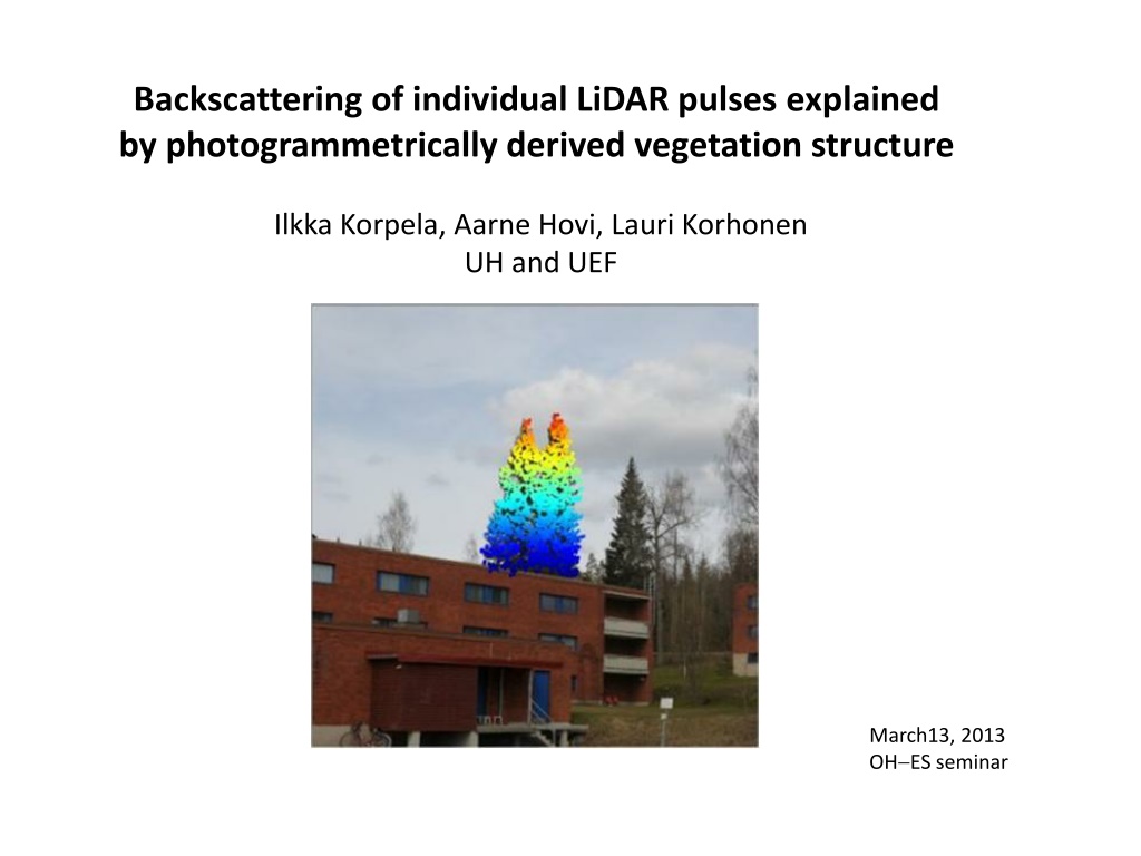
Backscattering of individual LiDAR pulses explained by photogrammetrically derived vegetation structure Ilkka Korpela, Aarne Hovi, Lauri Korhonen UH and UEF March13, 2013 OH ES seminar
Background Pulsed LiDAR sensors use time-stamped photons, short pulses are ranging devices are designed for topographic applications currently use a single and divergence r4 r3 r2 r1 Clock Laser PD WF digitizer AGC / amplifier 1. Leica ALS60, GPS/IMU & electronics. 2. Oscilloscopes for the AD conversion
Some basic features Overall HOT-SPOT view-illumination geometry, low . Transmitted pulse ~ P(t), t = 0...10 ns; stability is essential for radiometry iFOV ~ some mrads, (Q how is the iFOV weight function?) beam divergence 0.1-0.3 mrad Received P has PSun. Through a BPF and an aperture. (SNR) Receiver has a certain response; mapping input to output Signal has noise (speckle, photodiode, circuts, AD-conversion) Aperture of an ALS50-ii sensor. Oscillating mirror in resting position, collimating lens on the right.
Time-stamped photons on a deflected, yet known path scan zenith angles 0-20 mirror angle; GNSS / imu Pulse path < 0.2-0.4 m in XY, < 0.1 m in Z Gaussian PSF Intensity Perpendicular dist from cables, m
Vicarious refl. calibration for well-defined surfaces grass fine sand old asphalt bitumen Hemispherical conical reflectance factors @ 900 nm vs. 1064 nm backscattering (intensity) Flat ; 90 ; larger than footprint -surfaces
LiDAR challenging radiometry in vegetation Pine Birch Spruce Single pulse ~ stochastic Multiple pulses ~ structure, gaps, joint distributions , spatial dependencies, ... => constrain ill-posed nature
Wafeform sampling amplitude sequences Waveform, WF(t) is the output, affected by the system response, mm. Reflectance properties and orientation of the surface(s); their density and spatial configuration in the iFOV of P(t) + noise => contributions to WF(t) WFs tell more about the volumetric scattering than discrete peak amplitude data.
Experimental research Nominal scale * mature trees * understory trees * forest floor flora * mire flora samples Ratio scale? Viewing the pulse from its tail; what can we see and learn?
Geometry: 3D system of the images transformation to the 3D system of the LIDAR data Photogrammetric XYZ + ( X, Y, Z, rotation about Z) XYZ of LiDAR data Remnant offsets < 5 10 cm Camera positions XYknown XYknown XYknown ZLiDAR (known)
Remaining geometric LiDAR inaccuracy * Between-strip offsets and drifts * Short-term noise XY strip adjustment (local offset removal) using footprint silhouettes measured from the pulse tail -images, shifted ones. Correction for a site and LiDAR Strip.
XY LiDAR strip adjustment with detached branches Silhouette backscatter strength correlation peaked at some xy offset
Silhouette area vs. Backscattering Fig. 8b. Dependence between non-weighted relative silhouette area (0-1) and the intensity of the first return in the 60-yr-old pine stand. The figure shows data from a 1-km ALS60 strip (2012) and a 750-m Riegl LMS-Q680i strip that had been found the best xy-match.
Smallest echo/WF triggering targets? Adjacent path Pseudoechoes First echo or start-of-WF- recording
Some notes on results Close-range photogrammetry is feasible, an alternative to TLS (direct spherical). in-situ strip adjustment with branches,yes, but don t recommend Silhouette explains 50 90% of signal level (shallow targets, single species) Smallest objects in the upper canopy triggering an observation can be quite small Could not verify that E (W/m2) has a Gaussian spread across the footprint. Calibration for real silhouette > CC/LAI modeling What scatterers contributed to the WF, observable, to some degree
What next? Experimenting is tedious, slow and expensive, yet needed A good simulator would provide guidance (Aarne s talk), but that is tedious too (basic data on scattering, morphology) Interesting topics to look at (airborne LiDAR) Is the (long-term goal) idea of synthetic training data (imputation of LiDAR features) feasible with simulators? Multidivergent LiDAR data; better probing of canopy structure? WF analysis in tree species recognition, species is bottleneck How far from optimal are the current sensors? Role of passive multispectral data to be combined?