Stratospheric Aerosol Subtyping Confidence and Lidar Ratio Uncertainty

This research delves into the classification confidence of stratospheric aerosol subtypes and possibilities for quantifying uncertainties in lidar ratio estimates due to inaccurate classification. It discusses CALIOP initial aerosol lidar ratios, optical properties of stratospheric aerosol layers, classification based on color and depolarization ratios, and Gaussian fitting to measured properties.

• Stratospheric Aerosol
• Lidar Ratio
• Uncertainty Estimation
• CALIOP
• Aerosol Classification

vuk_can Follow

Uploaded on Sep 30, 2024 | 0 Views

Download Presentation

Please find below an Image/Link to download the presentation.

The content on the website is provided AS IS for your information and personal use only. It may not be sold, licensed, or shared on other websites without obtaining consent from the author. Download presentation by click this link. If you encounter any issues during the download, it is possible that the publisher has removed the file from their server.

Presentation Transcript

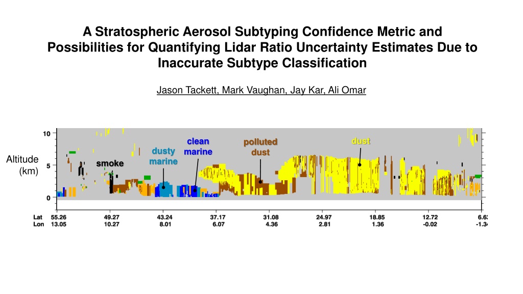
1. A Stratospheric Aerosol Subtyping Confidence Metric and Possibilities for Quantifying Lidar Ratio Uncertainty Estimates Due to Inaccurate Subtype Classification Jason Tackett, Mark Vaughan, Jay Kar, Ali Omar dust clean marine polluted dust dusty marine Altitude (km) smoke

2. CALIOP initial aerosol lidar ratios in V4.50 Subtype Clean marine Dust Polluted continental/smoke Clean continental Polluted dust Elevated smoke Dusty marine PSC aerosol Volcanic ash Sulfate Elevated smoke Unclassified 532 nm lidar ratio (sr) 23 5 44 9 70 25 53 24 55 22 70 16 37 15 50 10 61 17 50 18 70 16 50 18 1064 nm lidar ratio (sr) 23 5 44 13 30 14 30 17 48 24 30 18 37 15 50 10 44 13 30 14 30 18 30 14 Tropospheric aerosol Stratospheric aerosol

3. Stratospheric aerosol layer optical properties measured by CALIOP Ash Sulfate Smoke more Color Ratio Color Ratio Color Ratio Number of layers less Particulate Depolarization Ratio Particulate Depolarization Ratio Particulate Depolarization Ratio Histograms of manually classified aerosol layers with IAB > 0.001 /sr. Ash Sulfate Smoke Chait n 2008 Kasatochi 2008 Siberian wildfires 2007, 2012 Okmok 2008 Sarychev 2009 Canadian wildfires 2007, 2014 Contributing events: Puyehue-Cord n Caulle 2011 Nabro 2011 Pacific Northwest Event Aug. 2017 Calbuco 2015 Australian bush fires 2006, 2009

4. Stratospheric aerosol layer optical properties measured by CALIOP classification assigned Ash Sulfate Smoke more smoke ash ash smoke ash smoke Color Ratio Color Ratio Color Ratio Color Ratio Color Ratio Color Ratio Number of layers sulfate sulfate sulfate less Particulate Depolarization Ratio Particulate Depolarization Ratio Particulate Depolarization Ratio Particulate Depolarization Ratio Particulate Depolarization Ratio Particulate Depolarization Ratio Histograms of manually classified aerosol layers with IAB > 0.001 /sr. Thresholds in color ratio and depolarization ratio (black lines) are used to determine stratospheric aerosol subtype based on the distributions above.

5. Gaussian fit to measured properties Ash Sulfate Smoke 1 Color Ratio Color Ratio Color Ratio Color Ratio Color Ratio Color Ratio Frequency 0 Particulate Depolarization Ratio Particulate Depolarization Ratio Particulate Depolarization Ratio Particulate Depolarization Ratio Particulate Depolarization Ratio Particulate Depolarization Ratio Step 1: Fit distributions to cover all measurement space and normalize each distribution by maximum. ( ) ( ) ( ) n n X n X n X 1 2 3 = = = ( ) , ( ) , ( ) 3 n X n X n X 1 2 max( ) max( ) max( ) n n 1 2 3 feature = , X p

6. Stratospheric aerosol subtype confidence metric Ash Smoke Sulfate Color Ratio Color Ratio Color Ratio Color Ratio Color Ratio Color Ratio f ( , ) p Particulate Depolarization Ratio Particulate Depolarization Ratio Particulate Depolarization Ratio Particulate Depolarization Ratio Particulate Depolarization Ratio Particulate Depolarization Ratio Step 2: For each type, compute the differential occurrence probability against to the other two types: Interpretation of metric: For a given type classification, 2 n X + 1 + ( ) ( ) ) ( ) n X n X + ( ) ( ) P X ( ) ( ) X P X P P X = = ( ) P X , ( ) X 3 n P = 1 2,3 ( ) f X 1 2 3 1 2,3 ( n n 1 1 2,3 +1 = definitely the right type 1 = definitely some other type 0 = ambiguous classification Step 3: Weight by total number of samples: ( = , ) ( , ) ( f , ) f w ( ) X N N 1 1 p p p = ( ) w X sum max( ) sum

7. Puyhue-Cordn Caulle eruption, June 2011 (primarily ash) All stratospheric aerosol layers detected in southern hemisphere, excluding SAA Number of layers Highest confidence for ash initially, then similar confidence with smoke due to the allowance for depolarizing smoke in subtyping algorithm June July Confidence June July

8. Nabro eruption June 2011 (primarily sulfate) All stratospheric aerosol layers detected in northern hemisphere, excluding SAA Number of layers Highest confidence for sulfate June July August Confidence June July August

9. Australia bushfires, January 2020 All stratospheric aerosol layers detected in southern hemisphere, excluding SAA Number of layers Similar confidence for smoke and sulfate due to difficulty in separating these two types. January February Confidence January February

10. Can we use the aerosol subtype PDFs to estimate biases in lidar ratio selection? Ash Smoke Sulfate 1 Color Ratio Color Ratio Color Ratio Color Ratio Color Ratio Color Ratio n/max(n) 0 Particulate Depolarization Ratio Particulate Depolarization Ratio Particulate Depolarization Ratio Particulate Depolarization Ratio Particulate Depolarization Ratio Particulate Depolarization Ratio The lidar ratio bias is the deviation from the true lidar ratio. The PDFs indicate the probability of correct or incorrect classification. For a given subtype, the lidar ratio bias could be estimated as the sum of the lidar ratio errors for the other subtypes weighted by their probability of correct classification. ( ) ( ) n n X n X ( ) ( ) = + 3 S S S S S 2 1 1 2 1 3 max( ) max( ) n 2 3

11. Lidar ratio bias estimates due to incorrect subtype classification Ash classification S Sulfate classification S Smoke classification S Color Ratio Color Ratio Color Ratio Color Ratio Color Ratio Color Ratio S (sr) Particulate Depolarization Ratio Particulate Depolarization Ratio Particulate Depolarization Ratio Particulate Depolarization Ratio Particulate Depolarization Ratio Particulate Depolarization Ratio The lidar ratio bias is the deviation from the true lidar ratio. The PDFs indicate the probability of correct or incorrect classification. For a given subtype, the lidar ratio bias could be estimated as the sum of the lidar ratio errors for the other subtypes weighted by their probability of correct classification. ( ) ( ) n n X n X ( ) ( ) = + 3 S S S S S 2 1 1 2 1 3 max( ) max( ) n 2 3

12. Example 1. Ash-like measurements Ash classification S Sulfate classification S Smoke classification S Color Ratio Color Ratio Color Ratio Color Ratio Color Ratio Color Ratio S (sr) Particulate Depolarization Ratio Particulate Depolarization Ratio Particulate Depolarization Ratio Particulate Depolarization Ratio Particulate Depolarization Ratio Particulate Depolarization Ratio Default lidar ratios Ash = 61 sr Sulfate = 50 sr Smoke = 70 sr Tiny bias due to low probability of other subtypes with these measurements (noise or poor fit to histograms can cause this) S (sr) If classified as Ash Sulfate Smoke 0.1 9.0 +7.2 ( ) ( ) n n X n X ( ) ( ) = + 3 S S S S S 2 1 1 2 1 3 max( ) max( ) n 2 3

13. Example 2. Sulfate-like measurements Ash classification S Sulfate classification S Smoke classification S Color Ratio Color Ratio Color Ratio Color Ratio Color Ratio Color Ratio S (sr) Particulate Depolarization Ratio Particulate Depolarization Ratio Particulate Depolarization Ratio Particulate Depolarization Ratio Particulate Depolarization Ratio Particulate Depolarization Ratio Default lidar ratios Ash = 61 sr Sulfate = 50 sr Smoke = 70 sr S (sr) +7.1 If classified as Ash Sulfate Smoke Bias is large even though measurements are in center of sulfate distribution. This is because of the overlap with the smoke distribution. 8.4 +19.8 ( ) ( ) n n X n X ( ) ( ) = + 3 S S S S S 2 1 1 2 1 3 max( ) max( ) n 2 3

14. Example 3. Smoke-like measurements Ash classification S Sulfate classification S Smoke classification S Color Ratio Color Ratio Color Ratio Color Ratio Color Ratio Color Ratio S (sr) Particulate Depolarization Ratio Particulate Depolarization Ratio Particulate Depolarization Ratio Particulate Depolarization Ratio Particulate Depolarization Ratio Particulate Depolarization Ratio Default lidar ratios Ash = 61 sr Sulfate = 50 sr Smoke = 70 sr S (sr) If classified as Ash Sulfate Smoke 8.3 Slight high bias because of overlap with the smoke distribution. 18.6 +0.16 ( ) ( ) n n X n X ( ) ( ) = + 3 S S S S S 2 1 1 2 1 3 max( ) max( ) n 2 3

15. Summary Subtype confidence metric indicates probability that subtype is correct, incorrect, or ambiguous. Possibly a useful quality assurance metric. Requires training set of accurately classified layers machine learning is an option (e.g. Shan Zeng s work with fuzzy k-means). Adapting to tropospheric subtyping is more challenging. Lidar ratio biases can be estimated based on PDFs of measured properties. As above, requires a training set. How would they be reported in CALIOP products? Separate extinction uncertainty into two SDSs, one for random and one for systematic errors?