Understanding the Normal Distribution in Data Analysis
The normal distribution, also known as the bell-shaped or Gaussian distribution, is defined by the mean and standard deviation of quantitative data. It helps determine the range of values containing specific percentages of observations. Identifying frequency, probability, mean, and the relationship between mode, median, and mean are key concepts when analyzing normally distributed variables. Skewed distributions, positively or negatively skewed, exhibit more extreme values in one direction, affecting the shape of the curve.

Download Presentation

Please find below an Image/Link to download the presentation.
The content on the website is provided AS IS for your information and personal use only. It may not be sold, licensed, or shared on other websites without obtaining consent from the author. Download presentation by click this link. If you encounter any issues during the download, it is possible that the publisher has removed the file from their server.
E N D
Presentation Transcript
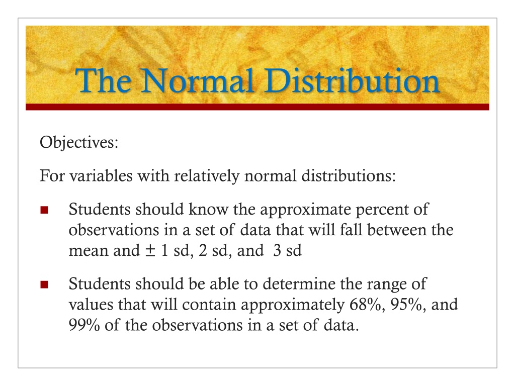
The Normal Distribution Objectives: For variables with relatively normal distributions: Students should know the approximate percent of observations in a set of data that will fall between the mean and 1 sd, 2 sd, and 3 sd Students should be able to determine the range of values that will contain approximately 68%, 95%, and 99% of the observations in a set of data.
The Normal Distribution (also called the bell-shaped or Gaussian distribution) Frequency or probability Mean
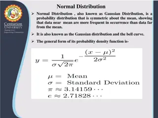
The Normal Distribution The normal distribution is completely defined by the mean and standard deviation of a set of quantitative data: The mean determines the location of the curve on the x axis of a graph The standard deviation determines the height of the curve on the y axis There are an infinite number of normal distributions- one for every possible combination of a mean and standard deviation
Examples of Normal Distributions Pr(X) on the y-axis refers to either frequency or probability.
Normal Distributions 25 20 Frequency Frequency 15 10 5 // 0 55 60 65 70 75 80 85 90 Heart Rate (BPM) Mean Many (but not all) continuous variables are approximately normally distributed. Generally, as sample size increases, the shape of a frequency distribution becomes more normally distributed.
Normal Distributions When data are normally distributed, the mode, median, and mean are identical and are located at the center of the distribution. Frequency of occurrence Mode, Median, Mean
Skewness Quantitative variables may also have a skewed distribution: When distributions are skewed, they have more extreme values in one direction than the other, resulting in a long tail on one side of the distribution. The direction of the tail determines whether a distribution is positively or negatively skewed. A positively skewed distribution has a long tail on the right, or positive side of the curve. A negatively skewed distribution has the tail on the left, or negative side of the curve.
Skewed Distributions Mode, Median, Mean Normal distribution Median Median Mode Mean Mode Mean Positively skewed distribution Negatively skewed distribution
Range of Observations For a normally distributed variable: ~68.3% of the observations lie between the mean and 1 standard deviation ~95.4% lie between the mean and 2 standard deviations ~99.7% lie between the mean and 3 standard deviations Mode, Median, Mean 68.3 % 95.4 % 99.7 % m-3s m-2s m-1s m m+1s m+2s m+3s
Heart Rate Example Sex HR Sex HR Sex HR Sex HR Sex HR Sex HR Sex HR F 55 M 66 F 70 M M 57 F 67 F 70 M M 59 F 67 M 70 M F 61 F 68 M 70 M M 61 F 68 F 71 F M 62 F 68 F 71 F M 62 M 68 M 71 F F 63 F 69 M 71 M F 64 M 69 F 72 F M 64 M 69 M 72 F M 64 M 69 F 73 M M 66 F 70 M 73 M For the heart rate data for 84 adults: 73 73 73 73 74 74 74 74 75 75 75 76 F F F M M F F F F M M M 77 77 77 77 77 78 78 78 78 78 78 79 M M M F F M F F F M F F 79 79 79 80 80 80 81 81 81 81 82 82 F M F M M F F M F F M M 82 82 83 83 83 84 84 85 86 86 89 89 Mean HR = 74.0 bpm SD = 7.5 bpm Mean 1SD = 74.0 7.5 = 66.5-81.5 bpm 25 Mean 2SD = 74.0 15.0 = 59.0-89.0 bpm 20 Frequency 15 10 Mean 3SD = 74.0 22.5 = 51.5-96.5 bpm 5 // 0 55 60 65 70 75 80 85 90 Heart Rate (BPM)
Heart Rate Example HR Data: 57/84 (67.9%) subjects are between mean 1SD 82/84 (97.6%) are between mean 2SD 84/84 (100%) are between mean 3SD 100 +3 SD 95 90 +2 SD 85 + 1SD Heart rate (bpm) 80 75 Mean 70 -1 SD 65 -2 SD 60 55 -3 SD 50 45 0 4 8 12 16 20 24 28 32 36 40 44 48 52 56 60 64 68 72 76 80 84 Subject number
Reference (Normal) Ranges in Medicine The normal range in medical measurements is the central 95% of the values for a reference population, and is usually determined from large samples representative of the population. The central 95% is approximately the mean 2 sd* Some examples of established reference ranges are: Serum Normal range fasting glucose sodium triglycerides 70-110 mg/dL 135-146 mEq/L 35-160 mg/dL Note: The value is actually 1.96 sd but for convenience this is usually rounded to 2 sd.
The Standard Normal Distribution A normal distribution with a mean of 0, and sd of 1 The distribution is also called the z distribution Any normal distribution can be converted to the standard normal distribution using the z transformation. Each value in a distribution is converted to the number of standard deviations the value is from the mean. The transformed value is called a z score.
Formula for the z transformation - m =x z s Once the data are transformed to z-scores, the standard normal distribution can be used to determine areas under the curve for any normal distribution.
Example of a z-transformation If the population mean heart rate is 74 bpm, and the standard deviation is 7.5, the z score for an individual with HR = 80 bpm is: - m - x 80 6 = = = = z 8 . 0 s The individual s HR of 80 bpm is 0.8 standard deviations above the mean.
Rule of Thumb #1 The z-value can be looked up in a table for the standard normal distribution to determine the lower and upper areas defined by a z-score of 0.8 (the areas are the lower 78.8% and upper 21.2%) You will not need to calculate z-scores or find corresponding areas under the curve for z-scores in this class, but you will be expected to know the following: The important z-scores to know are 1.645, 1.960*, 2.575 Note: when calculating by hand, it is OK to round 1.960 to 2
Rule of Thumb #2 The total area under the normal distribution curve is 1: 90% of the area is between 1.645 sd 95% of the area is between 1.960 sd 99% of the area is between 2.575 sd Area = 90% Area = 95% Area = 99% -2.575 -1.645 0 +1.645 +2.575 -1.960 +1.960
The Normal Distribution & Confidence Intervals 90% of the area is between 1.645 sd 95% of the area is between 1.960 sd 99% of the area is between 2.575 sd These are the most commonly used areas for defining Confidence Intervals which are used in inferential statistics to estimate population values from sample data


 Ranges in Medicine")