Understanding Ice Flow and Glacial Processes in Landscapes
Delve into the intricate world of ice flow and glacial processes, exploring topics such as the movement of ice sheets, effects of glacial erosion on topography, basal melt in ice sheets, and the formation of eskers. Discover the reasons behind U-shaped glacier-carved valleys, the role of water tables in glacier valleys, and the maintenance of subglacial conduits. Explore Mars examples and Earth examples to understand these phenomena better.

Download Presentation

Please find below an Image/Link to download the presentation.
The content on the website is provided AS IS for your information and personal use only. It may not be sold, licensed, or shared on other websites without obtaining consent from the author. Download presentation by click this link. If you encounter any issues during the download, it is possible that the publisher has removed the file from their server.
E N D
Presentation Transcript
GEOS 28600 The science of landscapes: Earth & Planetary Surface Processes http://geosci.uchicago.edu/~kite/geos28600_2019/ Lecture 6 Wednesday 30 Jan 2019 Wrap-up of The flow of ice Introduction to fluvial sediment transport
Logistics Homework 2 is due now No class next week due to NASA panel Homework 3 will be issued no later than next Mon and will be due in class on Mon 11 Feb
The flow of ice: why, how, and what are the effects? ICE MOVEMENT GLEN S LAW TEMPERATURE STRUCTURE WITHIN ICE SHEETS ESKERS (partly) EFFECT OF GLACIAL EROSION ON TOPOGRAPHY not yet
Wet-based ice sheets Basal melt Applications: ice streams will Greenland + Antarctic ice shelf collapse take a few millenia or a few centuries?
Eskers: sand+gravel ridges deposited from subglacial water channels Katahdin esker system, Maine Eskers can flow uphill: why?
How are subglacial conduits kept open? Viscous inflow of warm ice will seal conduits near the ocean interface in decades, unless opposed e.g. Rothlisberger 1972
Example: Mars, Dorsa Argentea Formation eskers (~3.5 Ga) Fastook et al. Icarus 2012 Butcher et al. Icarus 2016 South Pole of Mars
The flow of ice ICE MOVEMENT GLEN S LAW TEMPERATURE STRUCTURE WITHIN ICE SHEETS ESKERS (Mars examples) EFFECT OF GLACIAL EROSION ON TOPOGRAPHY (Earth examples)
Why are glacier- carved valleys U-shaped?
Origin of U-shaped glacial valleys: role of water table Harbor, 1992, GSA Bulletin
Glacial abrasion and plucking scales as (sliding velocity)2 using metamorphic grade of eroded rocks as a proxy for distance upstream Herman et al. Science 2015 Abrasion, quarrying
Global increase in erosion rate in the last 2 Myr possibly due to increase in glaciation Herman et al. Science 2013 (thermochronology compilation) For current state of debate, see Willenbring & Jerolmack Terra Nova 2016 (the case for steady erosion) and Herman & Champagnac Terra Nova 2016 (the case for last-2-Myr-increase in erosion) and Norton & Schlunegger Terra Nova 2017 (an insightful attempt to understand why the first two papers disagree).
Key points from The Flow of Ice: Glen s Law Approximations to the full Stokes equation: locations where they are and are not acceptable Nondimensional T-vs-depth as a function of accumulation rate for fixed basal heat flow Glacial erosion parameterization
Fluvial sediment transport: introduction REVIEW OF LAB 2 and REQUIRED READING (SCHOOF & HEWITT 2013) TURBULENT VELOCITY PROFILES, INITIATION OF MOTION BEDLOAD, RIVER GEOMETRY
Re << 1 inertial forces unimportant Stokes flow / creeping flow: Ice sheets can have multiple stable equilibria for the same external forcing, with geologically rapid transitions between equilibria Schoof & Hewitt 2013
Key points from Introduction to fluvial sediment transport : Critical Shields stress Differences between gravel-bed vs. sand-bed rivers Discharge-width scaling
Prospectus: fluvial processes Today: overview, hydraulics. Next lecture: initiation of motion, channel width adjustment. Channel long-profile evolution. Mountain belts. Looking ahead: landscape evolution (including fluvial processes.) This section of the course draws on courses by W.E. Dietrich (Berkeley), D. Mohrig (MIT U.T. Austin), and J. Southard (MIT).
Fluvial sediment transport: introduction REVIEW OF REQUIRED READING (SCHOOF & HEWITT 2013) TURBULENT VELOCITY PROFILES, INITIATION OF MOTION BEDLOAD, RIVER GEOMETRY
Hydraulics and sediment transport in rivers: 1) Relate flow to frictional resistance so can relate discharge to hydraulic geometry. 2) Calculate the boundary shear stress. Simplified geometry: average over a reach (12-15 channel widths). we can assume accelerations are zero. this assumption is better for flood flow (when most of the erosion occurs). riffle pool pool riffle Parker Morphodynamics e-book
The assumption of no acceleration requires that gravity (resolved downslope) balances bed friction. zx = ghsin averaging over 15-20 channel widths forces the water slope to ~ parallel the basal slope Dingman, chapter 6
Basal shear stress, frictional resistance, and hydraulic radius 1 z/h 0 b 0 At low slope (S, water surface rise/run), ~ tan ~ sin zx = ghsin b = gh S Frictional resistance: Boundary stress = ghsin L w Frictional resistance = b L (w + 2 h) h ghsin L w = b L (w + 2 h) w b = gh ( w / (w + 2 h ) ) sin Define hydraulic radius, R = hw / (w + 2 h) b = gR sin In very wide channels, R h (w >> h) L
Law of the wall, recap: Rivers ( Re >> 10, and fully turbulent): Glaciers ( Re << 1): zx = KT (du/dz) zx = (T, ) (du/dz) eddy viscosity, diffuses velocity Properties of turbulence: Irregularity Diffusivity Vorticity Dissipation From empirical & theoretical studies: KT = (k z )2 (du/dz) (where k = 0.39-0.4 = von Karman s constant) B = (k z)2 (du/dz)2 ( B / )1/2 = k z (du / dz) = u* = shear velocity ( g h S / )1/2 = u* = ( g h S )1/2 Memorize this. Now u* = k z (du / dz) Separate variables: du = (u* / k z ) dz Integrate: u = (u*/k) (ln z + c). For convenience, set c = -ln(z0) Then, u = (u*/k) ln (z/z0) law of the wall (explained on next slide) when z = z0, u = 0 m/s.
Calculating river discharge, Q (m3s-1), from elementary observations (bed grain size and river depth). u = (u*/k) ln (z/z0) law of the wall z0 is a length scale for grain roughness varies with the size of the bedload. In this class, use z0 = 0.12 D84, where D84 is the 84th percentile size in a pebble-count (100th percentile is the biggest). brackets denote vertical average Q = <u> w h h <u> = u(z) dz (1/(h-z0)) z0 <u> = (u*/k) (z0 + h ( ln( h / z0 ) 1 ) ) (1/ (h - z0)) h >> z0: Extending the law of the wall throughout the entire depth of the flow is a rough approximation do not use this for civil-engineering applications. This approach does not work at all when depth clast grainsize. <u> = (u*/k) ( ln( h / z0 ) 1 ) <u> = (u*/k) ln ( h / e z0) <u> = (u*/k) ln (0.368 h / z0) typically rounded to 0.4
Drag coefficient for bed particles: 3 alternative methods B = gRS = CD <u>2 / 2 <u> = ( 2g R S / CD )1/2 ( 2g / CD )1/2 = C = Chezy coefficient Chezy equation (1769) <u> = C ( R S)1/2 <u> = ( 8 g / f)1/2 ( R S )1/2 f = Darcy-Weisbach friction factor <u> = R2/3 S1/2 n-1 n = Manning roughness coefficient Most used, because lots of investment in measuring n for different objects 0.025 < n < 0.03 ----- Clean, straight rivers (no debris or wood in channel) 0.033 < n < 0.03 ----- Winding rivers with pools and riffles 0.075 < n < 0.15 ----- Weedy, winding and overgrown rivers n = 0.031(D84)1/6 ---- Straight, gravelled rivers In sand-bedded rivers (e.g. Mississippi), form drag due to sand dunes is important. In very steep streams, supercritical flow may occur: supercritical flow Fr # = <u>/(gh)1/2 > 1 Froude number
FL Sediment transport in rivers: (Shields number) At the initiation of grain motion, FD FD = ( F g FL ) tan tan FD/F g = 1 + (FL/FD) tan c D2 ( s )gD3 F g (submerged weight) = * c = ( s )gD Shields number ( drag/weight ratio ) Is there a representative particle size for the bedload as a whole? Yes: it s D50.
FL Equal mobility hypothesis FD Hiding effect small particles don t move significantly before the D50 moves. D/D50 Trade-off between size and embeddedness F g (submerged weight) Significant controversy over validity of equal mobility hypothesis in the late 80s early 90s. Parameterise using * = B(D/D50) = -1 would indicate perfect equal mobility (no sorting by grain size with downstream distance) = -0.9 found from flume experiments (permitting long-distance sorting by grain size).
*c50 ~ 0.04, from experiments (0.045-0.047 for gravel, 0.03 for sand) 1936: Hydraulically rough: viscous sublayer is a thin skin around the particles. sand gravel Re* = Reynolds roughness number 1999: Theory has approximately reproduced some parts of this curve. Causes of scatter: (1) differing definitions of initiation of motion (most important). (2) slope-dependence? (Lamb et al. JGR 2008) Buffington & Montgomery, Water Resources Research, 1999
Fluvial sediment transport: introduction REVIEW OF REQUIRED READING (SCHOOF & HEWITT 2013) TURBULENT VELOCITY PROFILES, INITIATION OF MOTION BEDLOAD, RIVER GEOMETRY
Consequences of increasing shear stress: gravel-bed vs. sand-bed rivers Suspension: characteristic velocity for turbulent fluctuations (u*) exceeds settling velocity (ratio is ~Rouse number). Typical transport distance 100m/yr in gravel-bedded bedload Sand: km/day John Southard (Experimentally, u* is approximately equal to rms fluctuations in vertical turbulent velocity) Empirically, rivers are either gravel-bedded or sand-bedded (little in between) The cause is unsettled: e.g. Jerolmack & Brzinski Geology 2010 vs. Lamb & Venditti GRL 2016
Bedload transport Meyer-Peter Muller Many alternatives, e.g. Yalin Einstein Discrete element modeling (Most common:) qbl = kb( b c)3/2 there is no theory for washload: it is entirely controlled by upstream supply John Southard
River channel morphology and dynamics Rivers are the authors of their own geometry (L. Leopold) And of their own bed grain-size distribution. Rivers have well-defined banks. Bankfull discharge 5-7 days per year; floodplains inundated every 1-2 years. Regular geometry also applicable to canyon rivers. Width scales as Q0.5 River beds are (usually) not flat. Plane beds are uncommon. Bars and pools, spacing = 5.4x width. Rivers meander. Wavelength ~ 11x channel width. River profiles are concave-up. Grainsize also decreases downstream.
Slope, grain size, and transport mechanism: strongly correlated z >20%; colluvial 8-20% boulder cascade (periodically swept by debris flows) 3-8% step-pool gravel bedload 0.1-3% bar-pool gravel bedload <0.1% bar-pool sand bedload & suspension rocks may be abraded in place; fine sediment bypasses boulders
What sets width? Q = wd<u> w = aQb d = cQf <u> = kQm b+f+m = 1 Comparing different points downstream b = 0.5 m = 0.1 f = 0.4 Eaton, Treatise on Geomorphology, 2013
What sets width? Three approaches to this unsolved question: (1) Posit empirical relationships between hydraulics, sediment supply, and form (Parker et al. 2008 in suggested reading; Ikeda et al. 1988 Water Resources Research). (2) Extremal hypotheses; posit an optimum channel, minimizing energy (Examples: minimum streampower per unit length; maximum friction; maximum sediment transport rate; minimum total streampower; minimize Froude number) (3) What is the actual mechanism? What controls what sediment does, how high the bank is, & c.?
Key points from Introduction to fluvial sediment transport Law of the wall how to calculate river discharge from elementary measurements (bed grain size and river depth). Critical Shields stress Differences between gravel-bed vs. sand-bed rivers Discharge-width scaling
Nye (1953) / Rothlisberger (1972) theory for subglacial conduits applications: plumbing system of cryovolcanoes on Enceladus and Ceres Assume: water temperature = ice temperature work done per unit volume of water per unit distance along flow pressure driving closure A,n: creep parameters for ice Energy required to raise water temperature (pressure dependence of the melting point of ice): melt-back rate warming of water heat generated by flow of water Following Cuffey, ch. 6., p.198-199 (suggested reading)
Pressure reduction in big Rothlisberger channels causes them to parasitize flow from smaller channels


, from elementary")


 / Rothlisberger (1972) theory for")