Foundations of Probability and Statistics

Probability theory provides mathematical models for chance processes, while statistics offers methods to test these models. This discipline finds diverse applications in fields like materials testing, quality control, production processes, and more. Understanding experiments, outcomes, and events is crucial in this domain. Probability distributions, random variables, and event operations are fundamental concepts in analyzing and interpreting data influenced by chance factors.

Download Presentation

Please find below an Image/Link to download the presentation.
The content on the website is provided AS IS for your information and personal use only. It may not be sold, licensed, or shared on other websites without obtaining consent from the author. Download presentation by click this link. If you encounter any issues during the download, it is possible that the publisher has removed the file from their server.
E N D
Presentation Transcript
Probability, Statistics Lecture-1 Additional chapters of mathematics Dmitriy Sergeevich Nikitin Assistant Tomsk Polytechnic University email: NikitinDmSr@yandex.ru 1
Rating plan for the discipline "Additional chapters of mathematics" Type of classes Estimated parameters Quantity Unit cost Total score 1. Lectures Visiting and lecture notes 12 0,5 6 Theoretical tests 4 5 20 2. Practical lessons Visiting and working 20 0,5 10 Control works 4 6 24 Individual homework 4 5 20 4. Exam 1) Theoretical question 2) Task 3) Task 20 (Extra points) - Report TOTAL (10) 100 (+10) 2
Probability, Statistics Probability theory provides models of probability distributions (theoretical models of the observable reality involving chance effects) to be tested by statistical methods, and it will also supply the mathematical foundation of these methods. Modern mathematical statistics has various engineering applications, for instance, in testing materials, control of production processes, quality control of production outputs, performance tests of systems, robotics, and automatization in general, production planning, marketing analysis, and so on. Although these applications are very heterogeneous, we will see that most statistical methods are universal in the sense that each of them can be applied in various fields. 3
Probability Theory If some numerical data are influenced by chance, by factors whose effect we cannot predict exactly (e.g., weather data, stock prices, life spans of tires, etc.), we have to rely on probability theory. It gives mathematical models of chance processes called random experiments or, briefly, experiments. In such an experiment we observe a random variable X, that is, a function whose values in a trial (a performance of an experiment) occur by chance according to a probability distribution that gives the individual probabilities with which possible values of Xmay occur in the long run. 4 4
Experiments, Outcomes, Events An experiment is a process of measurement or observation, in a laboratory, in a factory, on the street, in nature, or wherever; so experiment is used in a rather general sense. Our interest is in experiments that involve randomness, chance effects, so that we cannot predict a result exactly. A trial is a single performance of an experiment. Its result is called an outcome or a sample point. ntrials then give a sample of size nconsisting of nsample points. The sample space S of an experiment is the set of all possible outcomes. The subsets of Sare called events and the outcomes simple events. If, in a trial, an outcome a happens and a A (a is an element of A), we say that A happens. For instance, if a die turns up a 3, the event A: Odd number happens. 5
Unions, Intersections, Complements of Events The union ? ?of Aand Bconsists of all points in A or Bor both. The intersection ? ? of A and B consists of all points that are in both Aand B. If Aand Bhave no points in common, we write ? ? = where is the empty set (set with no elements) and we call A and B mutually exclusive (or disjoint) because, in a trial, the occurrence of A excludes that of B (and conversely). If your die turns up an odd number, it cannot turn up an even number in the same trial. Similarly, a coin cannot turn up Head and Tail at the same time. 6
Unions, Intersections, Complements of Events Complement ??of A. This is the set of all the points of S not in A. Thus ? ??= , ? ??= ? Another notation for the complement of A is ? (instead of??) but we will not use this because in set theory is used to denote the closure of A. Unions and intersections of more events are defined similarly. 7
Unions, Intersections, Complements of Events The union ? ??= ?? ?? ?? ?=? of events ??,?? ??consists of all points that are in at least one ??. Similarly for the union ?? ?? of infinitely many subsets ??,?? ??of an infinitesample space S(that is, Sconsists of infinitely many points). The intersection ? ??= ?? ?? ?? ?=? of ??,?? ??consists the points of Sthat are in each of these events. Similarly for the intersection ?? ?? of infinitely many subsets of S. 8
Unions, Intersections, Complements of Events Working with events can be illustrated and facilitated by Venn diagrams for showing unions, intersections, and complements, as in Figs., which are typical examples Fig. 1. Venn diagrams showing two events Aand Bin a sample space S and their union ? ?(colored) and intersection ? ?(colored) Fig. 2. Venn diagram for the experiment of rolling a die, showing S, A = {1, 3, 5}, C = {5, 6}, ? ? {1, 3, 5, 6}, ? ? {5} 9
Probability The probability of an event Ain an experiment is supposed to measure how frequently A is about to occur if we make many trials. If we flip a coin, then heads H and tails T will appear about equally often we say that H and T are equally likely. Similarly, for a regularly shaped die of homogeneous material ( fair die ) each of the six outcomes will be equally likely. Definition of Probability If the sample space Sof an experiment consists of finitely many outcomes (points) that are equally likely, then the probability of an event Ais ? ? =?????? ?? ????? ?? ? ?????? ?? ????? ?? ? 10
Axioms of probability Given a sample space S, with each event A of S (subset of S) there is associated a number called the probability of A, such that the following axioms of probability are satisfied. 1. For every Ain S, ? ? ? ?. 2. The entire sample space Shas the probability ? ? = ?. 3. For mutually exclusive events A and B (? ? = ) ? ? ? = ? ? + ?(?) 11
Basic Theorems of Probability T H E O R E M 1. Complementation Rule For an event A and its complement in a sample space S, ? ??= ? ? ? . T H E O R E M 2. Addition Rule for Mutually Exclusive Events For mutually exclusive events ??, ,??in a sample space S, ? ?? ?? ?? = ? ?? + ? ?? + + ? ??. T H E O R E M 3. Addition Rule for Arbitrary Events For events A and B in a sample space S, ? ? ? = ? ? + ? ? ? ? ? . 12
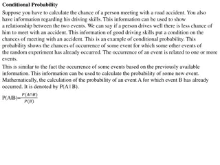
Conditional Probability Often it is required to find the probability of an event B under the condition that an event A occurs. This probability is called the conditional probability of B given A and is denoted by P(B|A). In this case A serves as a new (reduced) sample space, and that probability is the fraction P(A) of which corresponds to ? ?. Thus P(B|A) =? ? ? P(B|A) . ? ? Similarly, the conditional probability of A given B is P(A A| |B B) ) =? ? ? P( . ? ? T H E O R E M 4. Multiplication Rule. If A and B are events in a sample space S and ? ? ?,? ? ?, then ? ? ? = ? ? ? ?|? = ? ? ? ?|? . 13
Independent Events Independent Events. If events B and A are such that ? ? ? = ? ? ? ? they are called independent events. Assuming ? ? ?,? ? ?, P( P(A A| |B B) ) = ? ? , P( P(B B| |A A) ) = ? ? . This means that the probability of A does not depend on the occurrence or nonoccurrence of B, and conversely. This justifies the term independent. Independence of mEvents. Similarly, m events ??, ,?? are called independent if ? ?? ?? = ? ?? ? ??. 14
Random Variables. Probability Distributions A probability distribution or, briefly, a distribution, shows the probabilities of events in an experiment. The quantity that we observe in an experiment will be denoted by X and called a random variable (or stochastic variable) because the value it will assume in the next trial depends on chance, on randomness. If you roll a die, you get one of the numbers from 1 to 6, but you don t know which one will show up next. Thus Number a die turns up is a random variable. 15
Random Variables. Probability Distributions If we count (cars on a road, defective screws in a production, tosses until a die shows the first Six), we have a discrete random variable and distribution. If we measure (electric voltage, rainfall, hardness of steel), we have a continuous random variable and distribution. Precise definitions follow. In both cases the distribution of Xis determined by the distribution function (or cumulative distribution function) ? ? = ? ? ? ; this is the probability that in a trial, X will assume any value not exceeding x. 16
Random Variable A random variable X is a function defined on the sample space S of an experiment. Its values are real numbers. For every number a the probability ?(? = ?) with which Xassumes ais defined. Similarly, for any interval I the probability ?(? ?) with which Xassumes any value in Iis defined. The fundamental formula for the probability corresponding to an interval ? < ? ? ? ? < ? ? = ? ? ? ? . 17
Discrete Random Variables and Distributions By definition, a random variable Xand its distribution are discrete if Xassumes only finitely many or at most countably many values ??,??,??, , called the possible values of X, with positive probabilities ??= ? ? = ??,??= ?( ) ??,??= ? ? = ??, , whereas the probability ?(? ?) is zero for any interval I containing no possible value. ? = 18
Discrete Random Variables and Distributions Clearly, the discrete distribution of Xis also determined by the probability function f(x) of X, defined by ? ? = ?? ?? ? = ?? ? ????????? (? = ?,?, ) From this we get the values of the distribution function by taking sums, ? ? = ?(??) = ?? ?? ? ?? ? where for any given xwe sum all the probabilities ?? for which ?? is smaller than or equal to that of x. This is a step function with upward jumps of size ?? at the possible values ?? of Xand constant in between. 19
Discrete Random Variables and Distributions For the probability corresponding to intervals we have ? ? < ? ? = ? ? ? ? = ??. ?<?? ? This is the sum of all probabilities ?? for which ?? satisfies ? < ?? ?. From this and P(S)=1 we obtain the following formula (sum of all probabilities) ??= ?. ? 20
Continuous Random Variables and Distributions Discrete random variables appear in experiments in which we count (defectives in a production, days of sunshine in Chicago, customers standing in a line, etc.). Continuous random variables appear in experiments in which we measure (lengths of screws, voltage in a power line, Brinell hardness of steel, etc.). By definition, a random variable X and its distribution are of continuous type or, briefly, continuous, if its distribution function can be given by an integral ? ? ? = ? ? ?? whose integrand called the density of the distribution, is nonnegative, and is continuous, perhaps except for finitely many x-values. Differentiation gives the relation of f to F as ? ? = ? (?) for every xat which f(x) is continuous. 21
Discrete Random Variables and Distributions For the probability corresponding to intervals we have ? ? ? < ? ? = ? ? ? ? = ? ? ??. ? From this and P(S)=1 we obtain the following formula (sum of all probabilities) + ? ? ?? = ?. The next example illustrates notations and typical applications of our present formulas. 22
Discrete Random Variables and Distributions The mean characterizes the central location and the variance the spread (the variability) of the distribution. The mean (mu) is defined by = ???(??) (??? ???????? ????????????) ? + = ? ? ? ?? (??? ?????????? ????????????) and the variance (sigma square) by ?= (?? ?)??(??) (??? ???????? ????????????) ? + ?= (? ?)?? ? ?? (??? ?????????? ????????????) 23
Discrete Random Variables and Distributions (the positive square root of 2) is called the standard deviation of Xand its distribution. The mean is also denoted by E(X) and is called the expectation of Xbecause it gives the average value of Xto be expected in many trials. Quantities such as and 2 that measure certain properties of a distribution are called parameters. and 2 are the two most important ones. 2 >0 (except for a discrete distribution with only one possible value, so that 2 =0). We assume that and 2 exist (are finite), as is the case for practically all distributions that are useful in applications. 24
Theorems of Mean and Variance T H E O R E M 1. Mean of a Symmetric Distribution If a distribution is symmetric with respect to x = c, that is, f(c-x) = f(c+x), then = c T H E O R E M 2. Transformation of Mean and Variance If a random variable X has mean and variance 2, then the random variable ? = ??+ ??? has the mean * and variance *2, where = ??+ ?? and In particular, the standardized random variable Z corresponding to X, given by ? =? ? (??> ?). 2= ?????. ? has the mean 0 and the variance 1. 25
Expectation, Moments If g(x) is nonconstant and continuous for all x, then g(X ) is a random variable. Hence its mathematical expectation or, briefly, its expectation E(g(x)) is the value of g(x) to be expected on the average, defined + ?(??) ?(??) or ? = ?(? ? ) = ?(?) ? ? ?? ? In the first formula, fis the probability function of the discrete random variable X. In the second formula, fis the density of the continuous random variable X. Important special cases are the k-th moment of X(where k= 1, 2, ) + ?? ??? ? ?? ?(??) = ? ?(??) or ? = ? 26
Expectation, Moments and the k-th central moment of X (k = 1, 2, ) + ? ?(??)or ? = (? ?)?? ? ?? ? ? ??= ?? ? ? This includes the first moment, the mean of X = ?(?) It also includes the second central moment, the variance of X ??= ? ? ?? 27