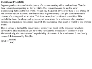
Understanding Conditional Probability and Bayes Theorem

Conditional probability explores the likelihood of event A given event B, while Bayes Theorem provides a method to update the probability estimate of an event based on new information. Statistical concepts such as the multiplication rule, statistical independence, and the law of total probability are crucial in these calculations. This content delves into examples and explanations to enhance your grasp of these fundamental probability principles.

Download Presentation

Please find below an Image/Link to download the presentation.
The content on the website is provided AS IS for your information and personal use only. It may not be sold, licensed, or shared on other websites without obtaining consent from the author. Download presentation by click this link. If you encounter any issues during the download, it is possible that the publisher has removed the file from their server.
E N D
Presentation Transcript
A Little Bit of Probability 3 Conditional Probability and Bayes Theorem
Conditional Probability Conditional probability: The probability of A given B The proportion of A and B in B Conditional operator | word flags : if, given, of the Pr(A) Note consequence: Pr(B)
Example In a large soil database 72% of the of the samples contain mica and 43% mica and schist. Assuming the database reflective of a relevant population, what is the probability that a randomly selected soil sample (from the same population) that contains mica also contains schist?
Example = 43% = 72% = 0.43/0.72 = 0.597 60% chance
Multiplication Rule Another important consequence of conditional probability is the multiplication rule:
Statistical Independence If A is independent of B then the probability of A is not affected by knowledge of B. If A and B are statistically independent if: If A and B do not satisfy the above they are statistically dependent
Example Using the information from the large soil database: 72% of the of the samples contain mica 43% contain mica and schist. 100% contain mica or schist Compute:
Example # Data from the question: M <- 0.72 # Schist MandS <- 0.43 # Mica and Schist # Pr(M) M # Pr(S|M) = Pr(SandM)/Pr(M) SgivenM <- MandS/M SgivenM # Pr(S and M) = Pr(M and S) MandS # Pr(S) = Pr(S or M) + Pr(S and M) - Pr(M) S <- 1 + 0.43 - 0.72 S # Pr(M|S) = Pr(M and S)/Pr(S) MgivenS <- 0.43/S MgivenS
The Law of Total Probability Suppose a sample space can be partitioned into a set of disjoint events Bi such that B4 B1 B3 A B2
The Law of Total Probability Suppose a sample space can be partitioned into a set of disjoint events Bi such that The probability of an arbitrary event A in can be written as: Law of total probability
Example: A medical test Professor P LOVES hamburgers. But he s also a hypochondriac. He thinks he is infected with Mad Cow Disease (MCD), so he gets himself tested (T). The true positive rate of the test is: Pr(T+ | MCD+) = 0.7 The false positive rate of the test is: Pr(T+ | MCD-) = 0.1 The background prevalence of MCD in the yummy cow population is: Pr(MCD+) = 0.02 What is the probability that Prof. P tests positive for MCD, Pr(T+)?
Example: A medical test # Data from the question: Tp.given.MCDp <- 0.7 Tp.given.MCDm <- 0.1 MCDp <- 0.02 # Pr(T+) = Pr(T+ | MCD+) Pr(MCD+) + Pr(T+ | MCD-) Pr(MCD-) Tp.given.MCDp * MCDp + Tp.given.MCDm * (1-MCDp)
Theres more than one way to condition: Bayes Theorem Intersection commutes: So: But from the multiplication rule we know: So: Bayes Theorem
Bayes Theorem A slightly more general form for Bayes Theorem: Suppose a sample space can be partitioned into a set of disjoint events Bi such that
Example: A medical test again Suppose Professor P is positive for MCD. What is the probability that he truly has MCD, Pr(MCD+| T+)? # Data from the question: Tp.given.MCDp <- 0.7 Tp.given.MCDm <- 0.1 MCDp <- 0.02 # Pr(T+) = Pr(T+ | MCD+) Pr(MCD+) + Pr(T+ | MCD-) Pr(MCD-) Tp <- Tp.given.MCDp * MCDp + Tp.given.MCDm * (1-MCDp) Tp # Pr(MCD+ | T+) = Pr(T+ | MCD+) Pr(MCD+) / Pr(T+) (Tp.given.MCDp * MCDp)/Tp