Evolution of Congestion Avoidance and Control Algorithms in Computer Networks
This content delves into the history of congestion collapse in computer networks and the pivotal role of Van Jacobson's congestion control algorithm. It discusses the reasons behind congestion collapse, the investigation into TCP behavior, and the steps taken to enhance TCP algorithms, emphasizing the conservation of packets principle. The impact of these developments on network performance is explored.

Download Presentation

Please find below an Image/Link to download the presentation.
The content on the website is provided AS IS for your information and personal use only. It may not be sold, licensed, or shared on other websites without obtaining consent from the author. Download presentation by click this link. If you encounter any issues during the download, it is possible that the publisher has removed the file from their server.
E N D
Presentation Transcript
Congestion Avoidance and Control Van Jacobson, Michael J. Karels Presenter: Shegufta Bakht Ahsan sbahsan2@Illinois.edu 09 October 2014
Published in ACM SIGCOMM, 1988 Citation Count : 6600+ This paper also has a big contribution on shaping the network today - HOW? We will explore it in today s presentation 2
Congestion Collapse Happens in a packet switched computer network Little or no useful communication happens due to congestion Generally occurs at Choke Points in the network Identified as a possible problem as far back as 1984 (RFC 896 , 6th January) First observed in the early Internet in October 1986 Data throughput from Lawrence Berkley Lab to UC Berkeley (separated by only 400 yards and two IMP hops !) dropped from 32 Kbps to 40 bps!!! Since then, it continued to occur until end nodes started implementing Van Jacobson s congestion control between 1987 and 1988 3
Congestion Collapse - Reason When more packets are sent than could be handled by intermediate routers, the intermediate routers discarded many packets expecting the end points of the network to retransmit the information Early TCP implementation had weird retransmission behavior ! When this packet loss occurred, the end points sent extra packets that repeated the information lost, doubling the data rate sent exactly the opposite of what should be done during congestion !!! This pushed the entire network into a congestion collapse where most packets were lost and the resultant throughput was negligible 4
Investigation !!! Was the 4.3BSD TCP misbehaving? YES Could it be tuned to work better under abysmal network conditions? YES 5
Steps Taken !!! Since that time, seven new algorithms were put into the 4BSD TCP: i. Round-trip-time variance estimation ii. Exponential retransmit timer backoff iii. Slow-start iv. More aggressive receiver ack policy v. Dynamic window sizing on congestion vi. Karn s clamped retransmit backoff vii. Fast retransmit We will focus on algorithm i to v, as they evolve from one common observation: The flow on a TCP connection should obey a conservation of packets principle 6
Conservation of Packets Conservation of packets means, connection is in equilibrium . In another word, a connection will run stably with a full window of data in transit. Such kind of transit is what a physicist would call conservative : A new packet isn t put into the network until an old packet leaves Packet conservation can be failed in only three ways: 1. The connection doesn t get to equilibrium, or 2. A sender injects a new packet before an old packet has exited, or 3. The equilibrium can t be reached because of resource limits along the path 7
Getting to Equilibrium: Slow-start Sender can use ACKs as a clock to strobe new packets into the network The receiver can not generate ACK faster than data packets get through the network, hence this protocol is self clocking 8
Getting to Equilibrium: Slow-start Figure 1 is a schematic representation of a sender and receiver on high bandwidth networks connected by a slower long-haul net The vertical dimension is bandwidth The horizontal dimension is time Each of the shaded box is a packet Bandwidth*Time = Bits, so the area of each box is the packet size Packet size does not change, hence a packet squeezed into the smaller long-haul bandwidth must spread out in time. 9
Getting to Equilibrium: Slow-start Sender has just started sending its first burst of packet back-to-back The ACK for the first of those packets is about to arrive back at the sender. Pb : minimum packet spacing on the slowest link Pr : incoming packet spacing in receiver side There is no queuing, therefore Pb = Pr 10
Getting to Equilibrium: Slow-start Ar : Spacing between ACKs on the receiver s side Ar = Pr = Pb Time Slot Pb is big enough for a packet, hence it would be big enough for ACK also. So the ACK spacing is preserved along the return path. Ab = Ar As: Spacing between ACKs on the sender s side As = Ab Hence, As = Pb 11
Getting to Equilibrium: Slow-start Hence, if packets after the first burst are sent only in response to an ACK, the sender s packet spacing will exactly match the packet time on the slowest link in the path BUT, how we will managethe first burst ? To get data flowing, there must be ACKs to clock out packets BUT to get ACKs there must be data flowing Sounds like the chicken or the egg problem ! 12
Getting to Equilibrium: Slow-start Slow Start algorithm: developed to start the clock by gradually increasing the amount of data in transit 1. Add a congestion window, cwnd, to the per-connection state 2. When starting or restarting after a loss, set cwnd to one packet 3. On each ACK for new data, increase cwnd by one packet 4. When sending, send the minimum of the receiver s advertised window and cwnd 13
Getting to Equilibrium: Slow-start One Round Trip Time 1 0th RTT One Packet Time 1st RTT 1 2 3 2nd RTT 3 2 6 7 4 5 3rd RTT 5 7 4 6 10 11 14 15 8 9 12 13 14
Getting to Equilibrium: Slow-start Slow start graduallyutilizes the channel s idle bandwidth According to the authors: Slow-start window increase isn t that slow: it takes Rlog2W where R is the round-trip-time and W is the window size in packets. This means, the window opens quickly enough to have a negligible effect on performance And the algorithm guarantees that, a connection will generate data at a rate at most twice the maximum possible on the path 15
Getting to Equilibrium: Slow-start On a side note: in the paper Why Flow-Completion Time is the Right metric for Congestion Control and why this means we need new algorithm , authors argue that TCP s slow-start mechanism increases the Flow Completion Time (FCT) Now a days, end-users are more interested to a network, which guarantees minimum FCT In this paper, authors explains how a new protocol called Rate Control Protocol (RCP) can achieve much better FCT than TCP or XCP 16
Getting to Equilibrium: Slow-start 65 155 17
Conservation at equilibrium: Round-Trip Timing Packet conservation can be failed in only three ways: 1. The connection doesn t get to equilibrium, or 2. A sender injects a new packet before an old packet has exited, or 3. The equilibrium can t be reached because of resource limits along the path Once data is flowing reliably, problem (2) and (3) should be addressed. 18
Conservation at equilibrium: Round-Trip Timing If the protocol is correct, (2) represent a failureof sender s retransmit timer. The TCP protocol specification suggests estimating mean round trip time via the low-pass filter R = R + (1- )M Where: R -> the average RTT estimate M -> round trip time measurement from the most recently acked data packet -> is a filter gain constant with a suggest value of 0.9 Once R estimate is updated, the retransmit timeout interval, RTO for the next packet is set to R accounts for the RTT variation 19
Conservation at equilibrium: Round-Trip Timing 20
Adapting to the path: congestion avoidance Packet conservation can be failed in only three ways: 1. The connection doesn t get to equilibrium, or 2. A sender injects a new packet before an old packet has exited, or 3. The equilibrium can t be reached because of resource limits along the path A timeout most probably indicates a lost packet, provided that the timers are in good shape Packets get lost for two reasons: 1. They are damaged in transit 2. The network is congested and somewhere on the path there is insufficient buffer capacity 21
Adapting to the path: congestion avoidance According to the authors, On most network paths, loss due to damage is rare (<<1%) ! Hence it is highly probable that a packet loss is due to a congestion in the network The congestion avoidance strategy should have two components: 1. The network must be able to signal the transport endpoints that congestion is occurring (or about to occur) 2. The end point must have a policy that decreases utilization if this signal is received and increases utilization if the signal isn t received 22
Adapting to the path: congestion avoidance In this scheme, if source detects a congestion, it will reduce its window size Wi = dWi-1 (d<1) It is a multiplicative decrease of the window size d is selected as 0.5 (WHY ?) 23
Adapting to the path: congestion avoidance Alice and Bob are equally sharing a 10Mbps channel If suddenly Alice shuts down her computer, 5Mbps bandwidth will be wasted unless Bob increases his window size and gradually capture the remaining idle bandwidth How to increase window size ? 24
Adapting to the path: congestion avoidance Should it be Wi = bWi-1, 1 < b < 1/d ? NO The result will oscillate wildly and on the average, deliver poor throughput Rather, this paper state that, the best increase policy is to make small, constant changes to the window size: Wi = Wi-1 + u u = 1 25
Adapting to the path: congestion avoidance Congestion Avoidance algorithm: 1. On any timeout, set cwnd to half the current window size (Multiplicative Decrease) 2. On each ACK for new data, increase cwnd by 1/cwnd (Additive Increase) 3. When sending, send the minimumof the receiver s advertised window and cwnd 26
Adapting to the path: congestion avoidance Packet conservation can be failed in only three ways: 1. The connection doesn t get to equilibrium, or 2. A sender injects a new packet before an old packet has exited, or 3. The equilibrium can t be reached because of resource limits along the path 27
Slow Start + Congestion Avoidance Sender keeps two state variables for congestion control: 1. A slow-start/congestion-avoidance window, cwnd 2. A threshold size, ssthresh to switch between two algorithm Sender always sends minimum of cwnd and the window advertised by the receiver On a timeout, half of the current window size is recorded in ssthresh (Multiple Decrease), after that cwnd is set to 1 ssthresh = cwnd/2; cwnd = 1; // initiates slow start 28
Slow Start + Congestion Avoidance When new data is ACKed, the sender does: if(cwnd < ssthresh) { cwnd += 1; // make cwnd double per RTT; multiplicative increase } else { cwnd += (1/cwnd); // increament cwnd by 1 per RTT, additive increase } 29
Slow Start + Congestion Avoidance One Round Trip Time 1 0th RTT One Packet Time 1st RTT 1 2 3 2nd RTT 3 2 6 * 4 * Current cwnd = 2 cwnd = cwnd + 1/cwnd = 2+ = 2.5 cwnd = cwnd + 1/cwnd = 2.5+ = 3 30
Evaluation Test setup to examine the interaction of multiple, simultaneous TCP conversations sharing a bottleneck link 1 MByte transfers (2048 512-data-byte packets) were initiated 3 seconds apart from four machines at LBL to four machines at UCB, one conversation per machine pair (the dotted lines above show the pairing) All traffic went via a 230.4 Kbps link The microwave link queue can hold up to 50 packets Each connection was given a window of 16 KB (32 512- byte packets) Thus any two connections could overflow the available buffering and the four connections exceeded the queue capacity by 160% 31
Evaluation 4,000 out of 11,000 packet sent were retransmission Among the 25KBps, one TCP conversation got 8KBps, two got 5KBps, one got 0.5KBps 32
Evaluation 89 out of 8281 packets were retransmitted Among the 25KBps, two TCP conversation got 8KBps and another two got 4.5KBps The difference between high and low bandwidth senders was due to the receivers. 33
Evaluation Normalized to the 25KBps link bandwidth Thin line without congestion avoidance: The sender send 25% more than link bandwidth Thick line with congestion avoidance The first 5 second is low: slow-start Large oscillation from 5 to 20: congestion control is searching for the correct window size Remaining time: run at the wire bandwidth Around 110: bandwidth re-negotiation due to the connection one shutting down 34
Evaluation Thin Line: without congestion avoidance. 75% bandwidth used for data, rest was used in retransmission Thick Line: with congestion avoidance 35
Thank You! Questions ? Increased Flow Completion Time TCP Global Synchronization Problem TCP RED (Random Early Detection) -Maybe we can try different initial values for cwnd and evaluate slow-start s performance in different settings.- 36