Parallel Prefix Networks in Divide-and-Conquer Algorithms
Explore the construction and comparisons of various parallel prefix networks in divide-and-conquer algorithms, such as Ladner-Fischer, Brent-Kung, and Kogge-Stone. These networks optimize computation efficiency through parallel processing, showcasing different levels of latency, cell complexity, and wiring patterns. Hybrid models like Brent-Kung/Kogge-Stone offer a balance between these factors. The content delves into the design principles and implementations of these networks, shedding light on their optimal delay characteristics.

Download Presentation

Please find below an Image/Link to download the presentation.
The content on the website is provided AS IS for your information and personal use only. It may not be sold, licensed, or shared on other websites without obtaining consent from the author. Download presentation by click this link. If you encounter any issues during the download, it is possible that the publisher has removed the file from their server.
E N D
Presentation Transcript
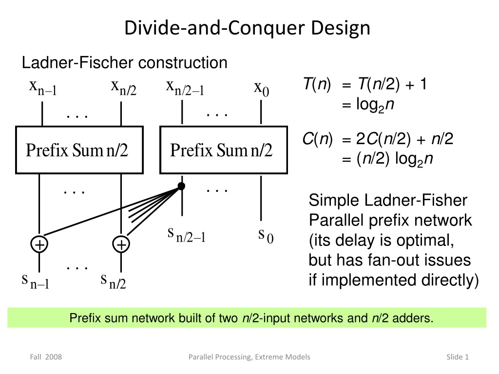
Divide-and-Conquer Design Ladner-Fischer construction xn 1 xn/2 xn/2 1 T(n) = T(n/2) + 1 = log2n C(n) = 2C(n/2) + n/2 = (n/2) log2n x0 . . . . . . Prefix Sum n/2 Prefix Sum n/2 . . . . . . Simple Ladner-Fisher Parallel prefix network (its delay is optimal, but has fan-out issues if implemented directly) sn/2 1 s0 + + . . . sn 1 sn/2 Prefix sum network built of two n/2-input networks and n/2 adders. Fall 2008 Parallel Processing, Extreme Models Slide 1
8.4 Parallel Prefix Networks xn 1xn 2 . . . x3x2x1x0 T(n) = T(n/2) + 2 = 2 log2n 1 C(n) = C(n/2) + n 1 = 2n 2 log2n + + + Prefix Sum n/2 This is the Brent-Kung Parallel prefix network (its delay is actually 2 log2n 2) + + sn 1sn 2 . . . s3s2s1s0 Fig. 8.6 Prefix sum network built of one n/2-input network and n 1 adders. Fall 2008 Parallel Processing, Extreme Models Slide 2
Example of Brent-Kung Parallel Prefix Network x15 x14 x13 x12 x11 x10 x9 x8 x7 x6 x5 x4 x3 x2 x1 x0 Originally developed by Brent and Kung as part of a VLSI-friendly carry lookahead adder One level of latency T(n) = 2 log2n 2 C(n) = 2n 2 log2n s15 s14 s13 s12 s11 s10 s9 s8 s7 s6 s5 s4 s3 s2 s1 s0 Brent Kung parallel prefix graph for n = 16. Fall 2008 Parallel Processing, Extreme Models Slide 3
Example of Kogge-Stone Parallel Prefix Network x15 x14 x13 x12 x11 x10 x9 x8 x7 x6 x5 x4 x3 x2 x1 x0 T(n) = log2n C(n) = (n 1) + (n 2) + (n 4) + ... + n/2 = n log2n n + 1 Optimal in delay, but too complex in number of cells and wiring pattern s15 s14 s13 s12 s11 s10 s9 s8 s7 s6 s5 s4 s3 s2 s1 s0 Kogge-Stone parallel prefix graph for n = 16. Fall 2008 Parallel Processing, Extreme Models Slide 4
Comparison and Hybrid Parallel Prefix Networks x15 x14 x13 x12 x15 x14 x13 x12 x11 x10 x9 x8 x11 x10 x9 x8 x7 x6 x5 x4 x3 x2 x1 x0 x7 x6 x5 x4 x3 x2 x1 x0 Brent/Kung 6 levels 26 cells Kogge/Stone 4 levels 49 cells s15 s14 s13 s12 s11 s10 s9 s8 s7 s6 s5 s4 s3 s2 s1 s0 s15 s14 s13 s12 s11 s10 s9 s8 s7 s6 s5 s4 s3 s2 s1 s0 x15 x14 x13 x12 x11 x10 x9 x8 x7 x6 x5 x4 x3 x2 x1 x0 Brent- Kung Fig. 8.10 A hybrid Brent Kung / Kogge Stone parallel prefix graph for n = 16. Kogge- Stone Han/Carlson 5 levels 32 cells Brent- Kung s15 s14 s13 s12 s11 s10 s9 s8 s7 s6 s5 s4 s3 s2 s1 s0 Fall 2008 Parallel Processing, Extreme Models Slide 5
Another Divide-and-Conquer Algorithm x0 x1 x2 x3 xn-2 xn-1 Parallel prefix computation on n/2 even-indexed inputs T(p) = T(p/2) + 1 Parallel prefix computation on n/2 odd-indexed inputs T(p) = log2p Strictly optimal algorithm, but requires commutativity Each vertical line represents a location in shared memory 0:0 0:2 0:n-2 0:1 0:3 0:n-1 Another divide-and-conquer scheme for parallel prefix computation. Fall 2010 Parallel Processing, Shared-Memory Parallelism Slide 6
n-th Root of Unity Xn = 1 nk+n/2 = = nk ndkd = = nk
DFT, DFT-1 O(n2)-time na ve algorithm using Horner-evaluation
Application of DFT to Smoothing or Filtering Input signal with noise DFT Low-pass filter Inverse DFT Recovered smooth signal Fall 2008 Parallel Processing, Extreme Models Slide 10
Application of DFT to Spectral Analysis 1 2 3 A 697 Hz 770 Hz 4 5 6 B Received tone 7 8 9 C 852 Hz DFT 941 Hz 0 # D * 1209 Hz 1336 Hz 1477 Hz 1633 Hz Tone frequency assignments for touch-tone dialing Frequency spectrum of received tone Fall 2008 Parallel Processing, Extreme Models Slide 11
Multiplying Two Polynomial [a0,a1,a2,...,an-1] [b0,b1,b2,...,bn-1] Pad with n 0's Pad with n 0's [a0,a1,a2,...,an-1,0,0,...,0] [b0,b1,b2,...,bn-1,0,0,...,0] DFT DFT [y0,y1,y2,...,y2n-1] [z0,z1,z2,...,z2n-1] Component Multiply [y0z0,y1z1,...,y2n-1z2n-1] inverse DFT [c0,c1,c2,...,c2n-1] (Convolution)
Fast Fourier Transform (FFT) yi = ui + ni vi (0 i < n/2) yi+n/2 = ui + ni+n/2 vi = ui - ni vi T(n) = 2T(n/2) + n = n log2n T(n) = T(n/2) + 1 = log2n in parallel sequentially Fall 2008 Parallel Processing, Extreme Models Slide 16
Computation Scheme for 16-Point FFT 0 1 2 3 4 5 6 7 8 9 0 1 2 3 4 5 6 7 8 9 0 0 4 0 0 2 4 6 0 0 4 0 0 1 2 3 4 5 6 7 0 0 4 10 11 12 13 14 15 10 11 12 13 14 15 j j 0 0 2 4 6 0 0 4 0 a + b a b a b j Butterfly operation Bit-reversal permutation Fall 2008 Parallel Processing, Extreme Models Slide 20
Parallel Architectures for FFT u0 y0 x0 y0 x0 u0 u1 y1 x4 x1 y4 u2 u2 y2 x2 x2 y2 u1 u3 y3 x3 x6 y6 u3 v0 y4 x4 x1 y1 v0 v1 y5 x5 x5 y5 v2 x6 v2 y6 x3 y3 v1 y7 x7 v3 x7 y7 v3 Butterfly network for an 8-point FFT. Parallel Processing, Extreme Models Slide 21


")
")
")
")
")