Understanding Binomial Distribution in R Programming
Probability distributions play a crucial role in data analysis, with the binomial distribution being a key one in R. This distribution helps describe the number of successes in a fixed number of trials with two possible outcomes. Learn about the properties, probability computations, mean, variance, and standard deviation associated with the binomial distribution. R provides built-in functions for working with this distribution, making it easier to analyze data effectively.
Download Presentation

Please find below an Image/Link to download the presentation.
The content on the website is provided AS IS for your information and personal use only. It may not be sold, licensed, or shared on other websites without obtaining consent from the author. Download presentation by click this link. If you encounter any issues during the download, it is possible that the publisher has removed the file from their server.
E N D
Presentation Transcript
Basic Probability Distributions in Basic Probability Distributions in R Programming R Programming By Dr. Mohamed Surputheen
probability distributions in R probability distributions in R Many statistical tools and techniques used in data analysis are based on probability. Probability measures how likely it is for an event to occur on a scale from 0 (the event never occurs) to 1 (the event always occurs). A probability distribution describes how a random variable is distributed; it tells us which values a random variable is most likely to take on and which values are less likely. R comes with built-in implementations of many probability distributions. Each probability distribution in R is associated with four functions which follow a naming convention: The d-prefix function calculates the probability density function (PDF) of a continuous probability distribution, or the probability mass function (PMF) of a discrete probability distribution, at a specific value of the random variable. The p-prefix function calculates the cumulative distribution function (CDF) of a probability distribution, which gives the probability of observing a value less than or equal to a given value of the random variable The q-prefix function calculates the quantile of a probability distribution, which is the inverse of the CDF. The r-prefix function generates random numbers from a probability distribution
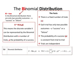
Binomial Distribution The binomial distribution is a discrete probability distribution that describes the number of successes in a fixed number of independent trials with two possible outcomes (success or failure) and a constant probability of success for each trial. A binomial experiment has the following properties: experiment consists of n identical and independent trials each trial results in one of two outcomes: success or failure P(success) = p P(failure) = q = 1 - p for all trials The random variable of interest, X, is the number of successes in the n trials. X has a binomial distribution with parameters n and p
Binomial Distribution If the probability of success in each trial is given by p , then the probability of getting exactly x successful events among n trials is given by the Binomial PMF or ! n = = x n x ( ) 1 ( ) for , 1 , 0 ..., P x p p x n x ( ! )! n x -n is the total number of trials -x is the number of successes -p is the probability of success on each trial.
Mean , variance and Standard deviation of Binomial Distribution The mean, E(X) = p + p + + p = n*p The variance, V(X) = pq + pq + + pq = n*pq The standard deviation =
Probability Computations Related to Binomial Distributions Probability Computations Related to Binomial Distributions R has several functions related to the binomial distribution. Here are some commonly used ones: 1. dbinom(x, size, prob) - Probability Mass Function (PMF) or probability distribution of the binomial distribution. Calculates the probability of getting exactly x successes in size trials, given a probability prob of success on each trial. 2. pbinom(q, size, prob) - Cumulative Distribution Function (CDF) of the binomial distribution. Calculates the probability of getting up to q successes in size trials, given a probability prob of success on each trial. 3. qbinom(p, size, prob) - Inverse CDF of the binomial distribution. Calculates the smallest number q such that the CDF is less than or equal to p, given size trials and a probability prob of success on each trial. (ie) This function takes the probability value and gives a number whose cumulative value matches the probability 4. rbinom(n, size, prob) - Random number generator for the binomial distribution. Generates n random samples from a binomial distribution with size trials and a probability prob of success on each trial.
Binomial probabilities using dbinom() function in R dbinom is the function used to find the probability mass function for the binomial distribution. The function dbinom is used to obtain the exact probability using Binomial distribution, i.e. P(X=x). The syntax to compute the probability at x for binomial distribution using R is dbinom(x,size,prob) where x : the value(s) of the variable, size : the number of trials, and prob : the probability of success (prob). The dbinom() function gives the probability for given value(s) x (no. of successes), size (no. of trials) and prob (probability of success).
Manual verification Example: dbinom The probability of getting a head on a single coin toss is 1/2, and the probability of getting a tail is also 1/2. A coin is tossed 5 times. What is the probability of getting one head and three heads? To solve this problem using R language, we can use the dbinom() function, which calculates the binomial probability mass function. To find the probability of getting a certain number of heads in 5 coin tosses, we can use the binomial probability formula: For getting one head: P(x) = nCx pxq(n-x) > dbinom(1, size=5, prob=0.5) Given n=5, p=0.5,q=0.5 [1] 0.15625 For getting three heads: So for getting one head, we have: P(X=1) = (5C1) * (1/2)^1 * (1/2)^4 = 5/32 =0.15625 > dbinom(3, size=5, prob=0.5) For getting three heads, we have: [1] 0.3125 P(X=3) = (5 C 3) * (1/2)^3 * (1/2)^2 = 10/32 = 5/16 =0.3125
Binomial cumulative probability using Binomial cumulative probability usingpbinom() pbinom() function in R function in R The syntax to compute the cumulative probability distribution function (CDF) for binomial distribution using R is pbinom(q,size,prob) where q : the value(s) of the variable, size : the number of trials, and prob : the probability of success (prob). This function is very useful for calculating the cumulative binomial probabilities for given value(s) of q (value of the variable x), size (no. of trials) and prob (probability of success).
In a university 45% of the students are female. A random sample of 10 students are selected. What is the probability that 2 or less female students are selected? Answer: pbinom(q,size,prob) pbinom(2,10,0.45) [1] 0.09955965
Binomial Distribution Quantiles using qbinom() in R qbinom is the R function that calculates the inverse CDF (or quqntiles) of the binomial distribution. W.k.t, This function takes the probability value and gives a number whose cumulative value matches the probability value. The syntax to compute the inverse CDF or quantiles of binomial distribution using R is qbinom(p,size,prob) where p : the value(s) of the probabilities, size : the number of trials, and prob : the probability of success (prob). Diff between CDF and invers CDF The CDF represents the probability that a random variable takes on a value less than or equal to a given value. The inverse CDF, on the other hand, does the opposite. It takes a probability as input and returns the value of the random variable that corresponds to that probability. The function qbinom(p,size,prob) gives the Inverse CDF of Binomial distribution for given value of p, size and prob. Note: qbinom is the inverse of the pbinom function. pbinom calculates the cumulative probability distribution function (CDF) of a binomial random variable, while qbinom calculates the inverse CDF or the quantile function of the binomial distribution.
Example problem that demonstrates the relationship between pbinom and qbinom: Suppose we flip a fair coin 10 times. What is the probability of getting 3 or fewer heads? To solve this problem using pbinom, we can set n = 10 and p = 0.5 (since the coin is fair) and use the following code: > pbinom(3, 10, 0.5) [1] 0.171875 This returns a probability of approximately 0.1719, meaning there is a 17.19% chance of getting 3 or fewer heads in 10 coin flips. To solve this problem using qbinom, we can again set n = 10 and p = 0.5 and use the following code: > qbinom( 0.171875, 10, 0.5) # This function takes the probability value and gives a number whose cumulative value matches the probability value. [1] 3 This returns a value of 3, which confirms that the probability of getting 3 or fewer heads is approximately 0.1719. Here, we used qbinom to find the value of k such that P(X k) = 0.1719.
Simulating Binomial random variable using Simulating Binomial random variable using rbinom rbinom() function in R () function in R The general R function to generate random numbers from Binomial distribution is rbinom(n,size,prob) where, n is the sample size, size is the number of trials, and prob is the the probability of success in binomial distribution. The function rbinom(n,size,prob) generates n random numbers from Binomial distribution with the number of trials size and the probability of success prob. Example: Generate 8 random values from a sample of 150 with probability of 0.4. > x <- rbinom(8,150,.4) > x [1] 61 51 54 54 56 62 62 48
Poisson Distribution Poisson Distribution The Poisson distribution is a probability distribution that describes the probability of a certain number of events occurring within a fixed time or space interval, given the average rate of occurrence( )of those events (ie) The Poisson distribution models the probability of a certain number of events occurring in a fixed interval of time, given the average rate at which the events occur. The binomial distribution models the probability of a fixed number of successes in a fixed number of independent trials, while the Poisson distribution models the probability of a fixed number of occurrences in a fixed time or space interval.
In 1837 French mathematician Simeon Dennis Poisson derived the distribution as a limiting case of Binomial distribution. It is called after his name as Poisson distribution. Conditions: (i) The number of trails n is indefinitely large i.e., n (ii) The probability of a success p for each trial is very small i.e., p 0 (iii) np= is finite (iv) Events are Independent
The random variable X is said to follow the Poisson probability distribution if it has the probability function: The pmf is given by P(X=x)= p(x) = e- x/ x! , for x=0,1,2 where P(x) = the probability of x successes over a given period of time or space, given = the expected number of successes per time > 0 e = 2.71828 (the base for natural logarithms) The mean of the distribution is . The variance of the distribution is also . The standard deviation of the distribution is .
Probability Computations Related to Poisson Distributions in R Probability Computations Related to Poisson Distributions in R In R, you can use the dpois(), ppois(), qpois(), and rpois() functions to work with the Poisson distribution. 1.dpois(x, lambda) calculates the Probability Mass Function (PMF) of the Poisson distribution at a specific value of x, given a Poisson parameter lambda. 2. ppois(q, lambda) calculates the Cumulative Distribution Function (CDF) of the Poisson distribution at a specific value of q, given a Poisson parameter lambda. 3. qpois(p, lambda) calculates the Inverse Cumulative Distribution Function (quantile function) of the Poisson distribution at a specific probability value p, given a Poisson parameter lambda. 4. rpois(n, lambda) generates n random samples from a Poisson distribution with a Poisson parameter lambda.
dpois The dpois function calculates the probability mass function for a Poisson distribution, given a particular value x and a parameter lambda. To solve this problem manually using the Poisson distribution, we can use the formula: dpois(x, lambda) x: number of successes P(X=x)= p(x) = e- x / x! lambda: average rate of success where lambda is the average number of events per interval (in this case, 10 customer calls per hour), x is the number of events we're interested in (in this case, 7 customer calls in the next hour), and e is the mathematical constant approximately equal to 2.71828. P(X = 7) = (e -10 * 10 7) / 7! = (0.0000454 * 10,000,000) / (7 * 6 * 5 * 4 * 3 * 2 * 1) = 0.09008 Therefore, the probability of receiving exactly 7 calls in the next hour is approximately 0.090 or 9.0%. Example: Suppose a call center receives an average of 10 customer calls per hour. What is the probability that the call center will receive exactly 7 calls in the next hour? Ans: > lambda <- 10 > x <- 7 > prob <- dpois(x, lambda) > prob [1] 0.09007923
ppois In R, you can use the ppois function to calculate the Cumulative Distribution Function (CDF) of the Poisson distribution. The CDF gives the probability of getting k or fewer events in a certain interval of time, given the average rate of events per unit time. ppois(q, lambda) q: number of successes lambda: average rate of success To solve this problem manually using the Poisson distribution, we can use the formula: P(X=x)= p(x) = e- x / x! where is the average rate of events per hour and x is the number of events. To find the probability of 4 or fewer births in an hour, we need to calculate the probabilities for k = 0, 1, 2, 3, and 4, and add them up: Examples: It is known that a certain hospital experience 4 births per hour. In a given hour, what is the probability that 4 or less births occur? P(0) = (40 * e (-4) )/ 0! = 0.0183 Answer: Using the Poisson Distribution with = 4 and x = 4, we find that P(X 4) = 0.62884. P(1) = (41 * e (-4))/ 1! = 0.0733 P(2) = (4 2 * e (-4) ) / 2! = 0.1465 > ppois(4,4) [1] 0.6288369 P(3) = (43 * e (-4) ) / 3! = 0.1953 So the probability of 4 or fewer births in an hour is approximately 0.6288 or 62.88%, which matches the result we obtained earlier. P(4) = (4 4 * e (-4) ) / 4! = 0.1953 Therefore, the probability of 4 or fewer births in an hour is: P(0 or 1 or 2 or 3 or 4) = P(0) + P(1) + P(2) + P(3) + P(4) = 0.6287
Qpois qpois is a function in the R programming language that calculates the inverse cumulative distribution function (also known as the quantile function) for the Poisson distribution. qpois(p, lambda) p: the probability value for which you want to find the Inverse CDF. lambda: the average rate of events per unit time. Example: Suppose that the number of people who visit a website in a day follows a Poisson distribution with a mean of 500 people. What is the minimum number of people that we can expect to visit the website in a day with a probability of at least 95%? To solve this problem using qpois, we can first find the Poisson distribution value that corresponds to a probability of 0.95 using the qpois function and the mean value of 500: > qpois(0.95, 500) [1] 537 This means that we can expect at least 537 people to visit the website in a day with a probability of at least 95%
rpois rpois is a function in R that generates random numbers from a Poisson distribution with a specified mean. The function takes two arguments: the number of random numbers to generate (n) and the mean of the Poisson distribution (lambda). rpois(n, lambda) n: number of random variables to generate lambda: mean of the Poisson distribution Example: suppose we want to generate 10 random numbers from a Poisson distribution with a mean of 5 > rpois(10, 5) [1] 5 3 8 2 6 6 4 2 3 8
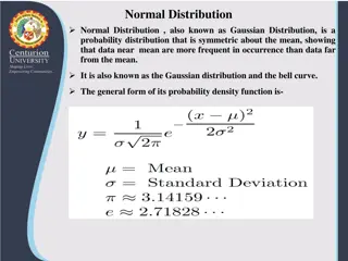
The Normal Distribution The Normal Distribution In probability theory and statistics, the Normal Distribution, also called the Gaussian Distribution, is the most significant continuous probability distribution. The normal distribution is a bell-shaped, symmetrical distribution(the values to the left of the mean are a mirror image of the values to the right of the mean.) in which the mean, median and mode are all equal. If the mean, median and mode are unequal, the distribution will be either positively or negatively skewed. A continuous random variable X having the bell-shaped distribution is called a normal random variable.
A random variable X is said to have a Normal distribution with parameters with mean and variance 2 if its probability density function is given by It is denoted by X ~ N ( , 2) Where f(x) = frequency of random variable x = 3.14159; e = 2.71828 = population standard deviation (> 0 ) x = value of random variable - < x < = population mean(- < < )
Properties of Normal Distribution Properties of Normal Distribution 1. It is a continuous distribution 2. The normal distribution curve is bell-shaped. 3. The mean, median, and mode are equal(Mean = Median = Mode = ) and located at the center of the distribution. 4. The normal distribution curve is unimodal (single mode). 5. The curve is symmetrical about the mean. (ie) Each half of the distribution is a mirror image of the other half. 6. It is asymptotic to the horizontal axis. That is, it does not touch the x-axis and it goes on forever in each direction. The random variable ?can take any value from ?? . 7. 8. The total area under the normal distribution curve is equal to 1 or 100%.(ie) 1 2?2(? ?)2?? = 1 ? ? ?? = ? 1 ? 2?
Standard Normal Distribution The simplest case of a normal distribution is known as the standard normal distribution. This is a special case when =0 and =1, and it is described by this probability density function. If X ~ N( , 2), let Z = (X - ) / , [Z-transformation] then E(Z) = 0, V (Z) = 1. (i.e)Z ~ N(0, 1), Z is said to have a standard normal distribution.
Probability Computations Related to Normal Distributions in R Probability Computations Related to Normal Distributions in R dnorm: density function of the normal distribution pnorm: cumulative density function of the normal distribution qnorm: quantile function of the normal distribution rnorm: random sampling from the normal distribution
Normal probabilities using Normal probabilities using dnorm dnorm dnorm() function in R () function in R The function dnorm returns the value of the probability density function (pdf) of the normal distribution given a certain random variable x, a population mean and population standard deviation . The syntax for using dnorm is as follows: dnorm(x, mean, sd) Manual verification The value of the density function at x=550 is Example: The GRE(Graduate Record Examinations ) is widely used to help predict the performance of applicants to graduate schools. The range of possible scores on a GRE is 200 to 900. The psychology department at a university finds that the students in their department have scores with a mean of 544 and standard deviation of 103. Find the value of the density function at x=550 > dnorm(550,544,103) [1] 0.00386666
Normal cumulative Density Function using pnorm() function in R The function pnorm returns the value of the Cumulative Density Function (CDF) of the normal distribution given a certain random variable q, a population mean and population standard deviation . The syntax for using pnorm is as follows: pnorm(q, mean, sd) (ie) pnorm is the cumulative density function for the normal distribution. By definition pnorm(x) = P(X x) Example : The GRE(Graduate Record Examinations ) is widely used to help predict the performance of applicants to graduate schools. The range of possible scores on a GRE is 200 to 900. The psychology department at a university finds that the students in their department have scores with a mean of 544 and standard deviation of 103. Find the probability that a student in psychology department has a score less than 480 we need to find the probability P(X 480) > pnorm(480,544,103) [1] 0.2671816
Normal Distribution Quantiles using qnorm() in R qnorm The function qnorm returns the value of the inverse cumulative density function (cdf) of the normal distribution given a certain random variable p, a population mean and population standard deviation . The syntax for using qnorm is as follows: qnorm(p, mean, sd) qnorm is the inverse function for pnorm. Example: Suppose that the heights of a certain population follow a normal distribution with a mean of 170 cm and a standard deviation of 5 cm. What is the height below which 90% of the population lies? > qnorm(0.9,170,5) [1] 176.4078 So the height below which 90% of the population lies is approximately 178.16 cm.
Simulating Normal random variable using rnorm() function in R rnorm is a function in R that generates random numbers from a normal distribution. rnorm(n, mean, sd) This function generates n random numbers from Normal distribution with given mean and sd rnorm generates random values from a standard normal distribution. The required argument is a number specifying the number of normal variates to produce. Example: generate 10 random numbers from a normal distribution with a mean of 5 and a standard deviation of 2: > rnorm( 10, 5, 2) [1] 7.448164 5.719628 5.801543 5.221365 3.888318 8.573826 5.995701 1.066766 [9] 6.402712 4.054417


