Understanding Binomial and Poisson Data Analysis
Discrete data, including Binomial and Poisson data, plays a crucial role in statistical analysis. This content explores the nature of discrete data, the concepts of Binomial and Poisson data, assumptions for Binomial distribution, mean, standard deviation, examples, and considerations for charting and interpreting data. It provides insights into using sample proportions, np-Charts, and sample size variations for effective analysis of Binomial data.
Download Presentation

Please find below an Image/Link to download the presentation.
The content on the website is provided AS IS for your information and personal use only. It may not be sold, licensed, or shared on other websites without obtaining consent from the author. Download presentation by click this link. If you encounter any issues during the download, it is possible that the publisher has removed the file from their server.
E N D
Presentation Transcript
Attributes Data Binomial and Poisson Data 1
Discrete Data All data comes in Discrete form. For Measurement data, in principle, it is on a continuous scale, but in reality it is truncated. As long as Sigma(X)>measurement unit, there is no problem with using charts. Count data, which occurs when counting Attributes, is discrete since we are restricted to Natural Numbers (0, 1, 2, etc.). 2
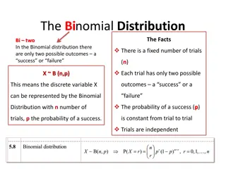
Binomial Data In SPC, Binomial Data usually arises when we count the number of items with a certain attribute, usuallythe number of defectives . Parts are tested and are either defective or not (sometimes called non-conforming ). In a sample of size n, we count the number of defectives. X=# of defectives in our sample, is our data. 3
If we have a Stable Process We can assume: Probability of a defective =p. Sample size is n. For Binomial data, this is referred to as the Area of Opportunity For all parts p is the same. Parts are defective or not independently of each other. 4
Binomial Distribution If our data satisfies those assumptions then our data, X, has a Binomial Distribution, i.e., ! n n k = = k P( ) (1 ) X k p p n k k ( )! ! 5
Mean and Standard Deviation The mean and standard deviation of X are: = ( ) E X np = ( ) (1 ) Sigma X np p 6
For Binomial data the sample size, or Area of Opportunity, may vary If the sample size is constant, then we can use an np-Chart since the Center Line will be a constant. If the sample size is not constant, then an np- Chart will have a non-constant centerline which makes the chart difficult to interpret. If we convert our data to sample proportions, the centerline is a constant, though the control limits are variable. 9
Sample Proportions used when the Area of Opportunity is not constant. The sample proportion is: = / p X n where = ( ) E p p and = ( ) (1 ) Sigma p p p n 10
Centerline and Control Limits Since we do not know the true value of p, we approximate it by using p-bar which will be the centerline for the p-chart, and for control limits we have (1 ) p p 3 p n i 11
We can plot the p-bar values with three sigma limits on a control chart. JMP with Example data: 12
When n is in the thousands: If n is in the thousands then almost no chart will show statistical control due to the tight limits since = ( ) (1 ) Sigma p p p n is so small. In this case an XmR chart gives a more reasonable estimate of Common Cause. 13
Examples where the attribute is not a defect Suppose you are examining order types (say categories of books) for Amazon. You may be interested in the proportion of children s books by month. You work for Menards and you want to look at the proportion of appliance orders by type by month. These proportions may vary naturally by month so should be included in Common Cause which an XmR chart will do. 14
Poisson Data Sometimes the product comes in units of length or area. In this case the non- conformities are counts which may be 0, 1, 2, which is different than Binomial Data where each item had a binary response. If the product can be considered an area for sampling purposes and the scattering of non- conformities can be considered random , then the data fits a Poisson Distribution. 15
Poisson Distribution The number of counts, X, of non-conformities in a unit is said to have a Poisson distribution with parameter lambda if k = = ( ) P X k e ! k 16
Mean and Standard Deviation The mean and standard deviation of X are given by: E(X)= and Sigma(X)= 17
Assumptions For data to be Poisson, it must satisfy some assumptions (we state in terms of area). Data is 0, 1, 2, The Expected number of counts in any area is proportional to the area size. The number of counts in any two disjoint areas are statistically independent. Probability theory then shows it must have the Poisson distribution. 18
Control charts for Poisson Data If the area sizes from which we take counts are all equal in size, that is, the Area of Opportunity is equal, then we may plot our sample data , , X X X ..... 1 2 3 on a control chart called a c chart (yes, c is for counts). 19
If lambda large enough If lambda is 20 or more the distribution is very symmetric and almost normally distributed and we can use three sigma limits in order to create a control chart. 23
Control limits for c chart We can get approximate limits for the c chart by using estimates of lambda since X and so three sigma limits should be 3 X X 24
Often the Area of Opportunity is not constant so we need to convert our data to rates If the area of opportunity is not constant we convert the counts to rates by dividing the counts by the area of opportunity and must use a u chart. u X = / a i i i 25
Centerline and control limits The centerline is given by u-bar which is the average rate per unit area n n = / u X a i i = = 1 1 i i with control limits u a 3 u i 26
Area of Opportunity and Control Limits For both the p-chart and u-chart, the Control Limits depend on two things: the rate of defects and the size of the Area of Opportunity. If the rate is higher, the variability is higher so the limits widen (we exclude the case for Binomial where p exceeds ). If the Area of Opportunity is larger the estimate of the rate is better so that the limits are narrower. 28
What happens when the defect rate is extremely low? When the defect rate is extremely low for Binomial or Poisson data, the three sigma limits have two problems with the charts: The data is so skewed that the limits are not correct. Any defect may show up as a signal the process is out of control. 29
For small lamda, around .01 or less Any defect will be outside of exact control limits. In this case the control limits will flag any defect as an out of control point. In this particular case, defect and out of control will coincide. Any defect will be investigated as Special Cause. There is no real consensus on this, but low defect rates are a problem anyone would like to have. 31


