Understanding Dynamic Channel Allocation in Computer Networks
Exploring the Data Link Layer and MAC Sublayer in computer networks, focusing on dynamic channel allocation, station models, collision assumptions, continuous vs. slotted time, carrier sense mechanisms, efficiency measurements, throughput calculation, media access strategies like channel partitioning and contention, and goals of contention MAC protocols for efficient medium sharing.

Uploaded on Sep 27, 2024 | 0 Views
Download Presentation

Please find below an Image/Link to download the presentation.
The content on the website is provided AS IS for your information and personal use only. It may not be sold, licensed, or shared on other websites without obtaining consent from the author. Download presentation by click this link. If you encounter any issues during the download, it is possible that the publisher has removed the file from their server.
E N D
Presentation Transcript
Computer Networks Lecture 6: Data Link layer >> MAC sublayer Based on slides from D. Choffnes Northeastern U. and P. Gill from StonyBrook University Revised Autumn 2015 by S. Laki
Dynamic Channel Allocation in LANs and MANs 1. Station Model. N terminals/hosts The prob. of a frame being generated in t is t, where the arrival rate is . 2. Single Channel Assumption. All stations are equivalent A single channel is available for all communications 3. Collision Assumption. If two frames are transmitted simultaneously, they overlap in time which results a garbled signal This event is called collision 4. Continuous Time VS Slotted Time. 5. Carrier Sense VS No Carrier Sense.
Dynamic Channel Allocation in LANs and MANs 4. Continuous Time VS Slotted Time. Time Time 5. Carrier Sense VS No Carrier Sense.
How can the efficiency be measured? Throughput (S) Number of packets/frames transmitted in a time unit (successfully) Delay The time needs for transmitting a packet Fairness All the terminals are treated as equals
Throughput and offered load Offered load (G) The number of packets in a time unit that the protocol must handle G>1: overloading An ideal protocol If G<1, S=G If G 1, S=1 where sending out a packet takes 1 time unit.
Strategies for Media Access 6 Channel partitioning Divide the resource into small pieces Allocate each piece to one host Example: Time Division Multi-Access (TDMA) cellular Example: Frequency Division Multi-Access (FDMA) cellular Taking turns Tightly coordinate shared access to avoid collisions Example: Token ring networks Contention Allow collisions, but use strategies to recover Examples: Ethernet, Wifi
Contention MAC Goals 7 Share the medium Two hosts sending at the same time collide, thus causing interference If no host sends, channel is idle Thus, want one user sending at any given time High utilization TDMA is low utilization Just like a circuit switched network Simple, distributed algorithm Multiple hosts that cannot directly coordinate No fancy (complicated) token-passing schemes
Contention Protocol Evolution 8 ALOHA Developed in the 70 s for packet radio networks Stations transmit data immedately If there is a collision, it retransmits the packet later. Slotted ALOHA Start transmissions only at fixed time slots Significantly fewer collisions than ALOHA Carrier Sense Multiple Access (CSMA) Start transmission only if the channel is idle CSMA / Collision Detection (CSMA/CD) Stop ongoing transmission if collision is detected
Pure ALOHA The goal was to use low-cost commercial radio equipment to connect users on Oahu and the other Hawaiian islands with a central time-sharing computer on the main Oahu campus. Algorithm was developed by Uni. of Hawaii If you have data to send, send the data Low-cost and very simple
ALOHA 10 Topology: radio broadcast with multiple stations Protocol: Stations transmit data immediately Receivers ACK all packets No ACK = collision, wait a random time then retransmit Simple, but radical concept Previous attempts all divided the channel TDMA, FDMA, etc. Optimized for the common case: few senders A B C
Performance analysis -Poisson Process The Poisson Process is a celebrated model used in Queuing Theory for random arrivals . Assumptions leading to this model include: The probability of an arrival during a short time interval t is proportional to the length of the interval, and does not depend on the origin of the time interval (memory-less property) The probability of having multiple arrivals during a short time interval t approaches zero.
Performance analysis - Poisson Distribution The probability of having k arrivals during a time interval of length t is given by: k t ( ) k t e = ( ) P t k ! where is the arrival rate. Note that this is a single- parameter model; all we have to know is .
FYI: Poisson Distribution 13 The following is the plot of the Poisson probability density function for four values of .
Analysis of Pure ALOHA Notation: Tf= frame time (processing, transmission, propagation) S: Average number of successful transmissions per Tf; that is, the throughput G: Average number of total frames transmitted per Tf D: Average delay between the time a packet is ready for transmission and the completion of successful transmission. We will make the following assumptions All frames are of constant length The channel is noise-free; the errors are only due to collisions. Frames do not queue at individual stations The channel acts as a Poisson process.
Analysis of Pure ALOHA Since Srepresents the number of good transmissions per frame time, and G represents the total number of attempted transmissions per frame time, then we have: S = G (Probability of good transmission) The vulnerable time for a successful transmission is 2Tf So, the probability of good transmission is not to have an arrival during the vulnerable time .
Analysis of Pure ALOHA 16 Collides with the start of the shaded frame Collides with the end of the shaded frame t t0 t0 + t t0 + 2t t0 + 3t Time Vulnerable Vulnerable period for the shaded frame
Analysis of Pure ALOHA Using: k t ( ) k t e = ( ) P t k ! And setting t = 2Tf and k = 0, we get 2 T 0 ( 2 ) T e f = = f 2 G (2 ) P T e 0 f 0! G T = = 2 G becasue . Thus, S G e f
Analysis of Pure ALOHA 18 If we differentiate S = Ge-2G with respect to G and set the result to 0 and solve for G, we find that the maximum occurs when and for that S = 1/2e = 0.18. So, the maximum throughput is only 18% of capacity. G = 0.5,
Tradeoffs vs. TDMA 19 In TDMA, each host must wait for its turn Delay is proportional to number of hosts In Aloha, each host sends immediately Much lower delay But, much lower utilization Throughput ALOHA Frame Sender A ALOHA Frame Sender B Time Load Maximum throughput is ~18% of channel capacity
Slotted ALOHA 20 Channel is organized into uniform slots whose size equals the frame transmission time. Transmission is permitted only to begin at a slot boundary. Here is the procedure: While there is a new frame A to send do Send frame A at (the next) slot boundary
Analysis of Slotted ALOHA Note that the vulnerable period is now reduced in half. Using: ( ) ( t P k = k t ) k t e ! And setting t = Tf and k = 0, we get T 0 ( ) T e f = = f G ( ) P T e 0 f 0! G T = = G because . Thus, S G e f
Slotted ALOHA 22 Protocol Same as ALOHA, except time is divided into slots Hosts may only transmit at the beginning of a slot Thus, frames either collide completely, or not at all 37% throughput vs. 18% for ALOHA But, hosts must have synchronized clocks Throughput Load
Broadcast Ethernet 24 Originally, Ethernet was a broadcast technology 10Base2 Terminator Repeater Tee Connector Hubs and repeaters are layer-1 devices, i.e. physical only 10BaseT and 100BaseT T stands for Twisted Pair Hub
Carrier Sense Multiple Access (CSMA) Additional assumption: Each station is capable of sensing the medium to determine if another transmission is underway
Non-persistent CSMA While there is a new frame A to send Check the medium If the medium is busy, wait some time, and go to 1. (medium idle) Send frame A 1. 2. 3.
1-persistent CSMA While there is a new frame A to send 1. Check the medium 2. If the medium is busy, go to 1. 3. (medium idle) Send frame A
p-persistent CSMA While there is a new frame A to send Check the medium If the medium is busy, go to 1. (medium idle) With probability p send frame A, and probability (1- p) delay one time slot and go to 1. 1. 2. 3.
CSMA Summary 29 Nonpersistent 1-persistent p-persistent CSMA persistence and backoff Non-persistent: Transmit if idle Otherwise, delay, try again Constant or variable Delay Time Channel busy Ready 1-persistent: Transmit as soon as channel goes idle If collision, back off and try again p-persistent: Transmit as soon as channel goes idle with probability p Otherwise, delay one slot, repeat process
Persistent and Non-persistent CSMA Comparison of throughput versus load for various random access protocols.
CSMA with Collision Detection Stations can sense the medium while transmitting A station aborts its transmission if it senses another transmission is also happening (that is, it detects collision) Question: When can a station be sure that it has seized the channel? Minimum time to detect collision is the time it takes for a signal to traverse between two farthest apart stations.
CSMA/CD A station is said to seize the channel if all the other stations become aware of its transmission. There has to be a lower bound on the length of each frame for the collision detection feature to work out. Ethernet uses CSMA/CD
CSMA/CD 33 Carrier sense multiple access with collision detection Key insight: wired protocol allows us to sense the medium Algorithm Sense for carrier If carrier is present, wait for it to end Sending would cause a collision and waste time Send a frame and sense for collision If no collision, then frame has been delivered If collision, abort immediately Why keep sending if the frame is already corrupted? Perform exponential backoff then retransmit 1. 2. 3. 4. 5. 6.
CSMA/CD Collisions 34 Spatial Layout of Hosts Collisions can occur Collisions are quickly detected and aborted A B C D Note the role of distance, propagation delay, and frame length t0 t1 Time Detect Collision and Abort
Exponential Backoff 35 When a sender detects a collision, send jam signal Make sure all hosts are aware of collision Jam signal is 32 bits long (plus header overhead) Exponential backoff operates: Select k [0, 2n 1] unif. rnd., where n = number of collisions Wait k time units (packet times) before retransmission n is capped at 10, frame dropped after 16 collisions Backoff time is divided into contention slots Remember this number
Minimum Packet Sizes 36 Why is the minimum packet size 64 bytes? To give hosts enough time to detect collisions What is the relationship between packet size and cable length? A B 1. Time t: Host A starts transmitting 2. Time t + d: Host B starts transmitting 3. Time t + 2*d: collision detected Basic idea: Host A must be transmitting at time 2*d! Propagation Delay (d)
CSMA/CD CSMA/CD can be in one of three states: contention, transmission, or idle. To detect all the collisions we need Tf 2Tpg where Tf is the time needed to send the frame And Tpg is the propagation delay between A and B
Minimum Packet Size 38 Host A must be transmitting after 2*d time units Min_pkt = rate (b/s) * 2 * d (s) but what is d? propagation delay: limited by speed of light Propagation delay (d) = distance (m) / speed of light (m/s) This gives: Min_pkt = rate (b/s) * 2 * dist (m) / speed of light (m/s) faster Ethernet standards 10 Mbps Ethernet Packet and cable lengths change for So cable length is equal . Dist = min_pkt * light speed /(2 * rate) (64B*8)*(2.5*108mps)/(2*107bps) = 6400 meters
Cable Length Examples 39 min_frame_size*light_speed/(2*bandwidth) = max_cable_length (64B*8)*(2.5*108mps)/(2*10Mbps) = 6400 meters What is the max cable length if min packet size were changed to 1024 bytes? 102.4 kilometers What is max cable length if bandwidth were changed to 1 Gbps ? 64 meters What if you changed min packet size to 1024 bytes and bandwidth to 1 Gbps? 1024 meters
Maximum Packet Size 40 Maximum Transmission Unit (MTU): 1500 bytes Pros: Bit errors in long packets incur significant recovery penalty Cons: More bytes wasted on header information Higher per packet processing overhead Datacenters shifting towards Jumbo Frames 9000 bytes per packet
Long Live Ethernet 41 Today s Ethernet is switched More on this later 1Gbit and 10Gbit Ethernet now common 100Gbit on the way Uses same old packet header Full duplex (send and receive at the same time) Auto negotiating (backwards compatibility) Can also carry power
Just Above the Data Link Layer 42 Bridging How do we connect LANs? Application Presentation Session Transport Network Data Link Physical Function: Route packets between LANs Key challenges: Plug-and-play, self configuration How to resolve loops
Recap 43 Originally, Ethernet was a broadcast technology Terminator Repeater Tee Connector Hub Pros: Simplicity Hardware is stupid and cheap Cons: No scalability More hosts = more collisions = pandemonium
Bridging the LANs 44 Hub Hub Bridging limits the size of collision domains Vastly improves scalability Question: could the whole Internet be one bridging domain? Tradeoff: bridges are more complex than hubs Physical layer device vs. data link layer device Need memory buffers, packet processing hardware, routing tables
Bridges 45 Original form of Ethernet switch Connect multiple IEEE 802 LANs at layer 2 1. Forwarding of frames 2. Learning of (MAC) Addresses 3. Spanning Tree Algorithm (to handle loops) Goals Reduce the collision domain Complete transparency Plug-and-play, self-configuring No hardware of software changes on hosts/hubs Should not impact existing LAN operations Hub
Frame Forwarding Tables 46 Each bridge maintains a forwarding table MAC Address Port Age 00:00:00:00:00:AA 1 1 minute 00:00:00:00:00:BB 2 7 minutes 00:00:00:00:00:CC 3 2 seconds 00:00:00:00:00:DD 1 3 minutes
Learning Addresses 47 Manual configuration is possible, but Time consuming Error Prone Not adaptable (hosts may get added or removed) Delete old entries after a timeout Instead, learn addresses using a simple heuristic Look at the source of frames that arrive on each port MAC Address Port Age 00:00:00:00:00:AA 1 0 minutes 00:00:00:00:00:AA 00:00:00:00:00:BB 2 0 minutes Port 1 Port 2 00:00:00:00:00:BB Hub
The Danger of Loops 48 CC DD <Src=AA, Dest=DD> This continues to infinity How do we stop this? Remove loops from the topology Without physically unplugging cables 802.1 (LAN architecture) uses an algorithm to build and maintain a spanning tree for routing Hub Port 2 Port 2 AA AA AA 1 2 1 AA AA AA 1 2 1 Port 1 Port 1 Hub AA BB
Spanning Tree Definition 49 A subset of edges in a graph that: Span all nodes Do not create any cycles 5 This structure is a tree 1 1 2 2 3 3 4 6 2 3 5 5 1 4 4 7 6 6 7 7
802.1 Spanning Tree Approach 50 Elect a bridge to be the root of the tree Every bridge finds shortest path to the root Union of these paths becomes the spanning tree 1. 2. 3. Bridges exchange Configuration Bridge Protocol Data Units (BPDUs) to build the tree Used to elect the root bridge Calculate shortest paths Locate the next hop closest to the root, and its port Select ports to be included in the spanning trees
Determining the Root 51 Initially, all hosts assume they are the root Bridges broadcast BPDUs: Bridge ID Root ID Path Cost to Root Based on received BPDUs, each switch chooses: A new root (smallest known Root ID) A new root port (what interface goes towards the root) A new designated bridge (who is the next hop to root)


")