Groundwater Flow: Assumptions, Solutions, and Tests
Explore basic assumptions, solutions, and tests related to groundwater flow in aquifers, including confined and unconfined scenarios. Learn concepts such as Thiem solution, Theis solution, and data analysis from pumping tests.

Download Presentation

Please find below an Image/Link to download the presentation.
The content on the website is provided AS IS for your information and personal use only. It may not be sold, licensed, or shared on other websites without obtaining consent from the author. Download presentation by click this link. If you encounter any issues during the download, it is possible that the publisher has removed the file from their server.
E N D
Presentation Transcript
+ Review Session 2 Flow to Wells
+Know at least a few of these Basic Assumptions (3-5) Aquifer bounded on the bottom Horizontal Geologic Formations (with infinite extent) The potentiometric surface is horizontal and is steady prior to pumping Any changes in potentiometric surfaces are due to pumping Aquifer is homogeneous and isotropic All flow is radial towards the well Groundwater flow is horizontal Darcy s Law is valid Water has constant density and viscosity Wells are fully penetrating Pumping well has infinitesimal diameter and 100 efficiency
+Steady State Confined Aquifer (Thiem solution) Q lnr2 T = 2p h2-h1 ( ) r1 Q is volume flow rate of well r1 is radius from pumping well to observation well 1 Know how to translate depth to water information into head differences r2 is radius from pumping well to observation well 2 h1 is head at well 1 i.e. h2-h1=d1-d2 h2 is head at well 2
+Steady State Unconfined Aquifer (Thiem solution) Q 2-b2 lnr2 K = p b2 ( ) r1 1 H Q is volume flow rate of well r1 is radius from pumping well to observation well 1 Know how to translate depth to water (d) information into heads r2 is radius from pumping well to observation well 2 b1= H-d1 b2=H-d2 b1 is head at well 1 You need to know depth of aquifer H b2 is head at well 2
+Flow in a Completely Confined Aquifer Theis Solution Additional Assumptions (Again know these) Aquifer is confined on top and bottom No recharge Aquifer is compressible and water is released instantaneously Well is pumped at a constant rate
+Data from a pumping test Q is volume flow rate of well r1 is radius from pumping well to observation well 1 Time when line intersects x axis Kb=T =0.1833Q S =2.246Tt* Ds10 r2 Change in drawdown over one decade on log scale
+Overlay the Two and pick a match point (does not have to be on the curves usually 1,1 on well function curve) S =4Tut Q )W u ( ) T = 4p h -h0 ( r2 Typically we pick match point such that W(u)=1 and u=1 Q is volume flow rate of well r is radius from pumping well to observation well h-h0 is drawdown on data at match point t is time on data plot at the match point
+Slug Tests The Poor Mans Alternative Pumping Tests are expensive for many many reasons (labor costs, well drilling costs, equipment, etc.). Sometime one way also not actually wish to extract water from an aquifer for fear that it may be contaminated. Slug Tests (or their counterpart bail-down tests) are a cheap and quick alternative A known quantity of water is quickly added or removed from a well and the response of water level in the well is measured. Water does not have to be added instead a slug of known volume can be thrown in, displacing a known volume of water. Slug test responses can be overdamped or underdamped and different and appropriate methods must be chosen to properly analyse data.
+Overdamped Cooper-Bredehoeft-Papadopulos ( )/rs T =rc 2/t1 S = rc 2m 2 rc is well casing radiius rs is well screen radius corresponds to best match curve (log10 mu=??) t1 is the time on real data curve where on the type curve Tt/rc2=1 on best match type curve
+Overlay Graphics Tt/rc2=1 on type curve plot
+Remove the Type Curve, but keep vertical line When overlaid on Figure 5.19 We identify mu=1e-6 (see figure below) t1=0.1 t1=0.1
+Overdamped Hvorslev Method If the length of the piezometer is more than 8 times the radius of the well screen, i.e. Lc/R>8 then ( 2Let37 ) K =r2ln Le/ R K hydraulic conductivity r radius of the well casing R radius of the well screen Le length of the well screen t37 time it take for the water level to rise or fall to 37% of the initial change.
+Overdamped Hvorslev Method Interpretation If the length of the piezometer is more than 8 times the radius of the well screen, i.e. Lc/R>8 then ( ) K =r2ln Le/ R 2Let37 K hydraulic conductivity r radius of the well casing R radius of the well screen Le length of the well screen t37 time it take for the water level to rise or fall to 37% of the initial change.
+Underdamped Van der Kamp T =c+aln T ( ) 2p t2-t1 =2p Dt w = g g g/L L = d = v2+g2 g =ln H t1 ( )/H t2 ( ) t2-t1 2 g/L 8d a=rc c=-aln 0.79rs 2S g/L Then ( ) T0=c+aln c ( ) ( ) T2=c+aln T1 T1=c+aln T0 Until converged
+Cautions and Guidelines for Slug Tests (Know these) Skin Effects can yield underpredictions Geological Survey Guidelines Three or more slug tests should be performed on a given well Two or more different initial displacement should be used The slug should be introduced as instantaneously as possible Good data acquisition equipment should be used An observation well should be employed for storage estimation Analysis method should be consistent with site Study results carefully and reassess analysis method if necessary Appropriate well construction parameters should be used