Power System Analysis Lecture: Transient Stability with Prof. Tom Overbye

In Lecture 23 of ECE 476, Prof. Tom Overbye discusses transient stability in power systems. Topics include power system time scales, frequency variations, dynamics behavior, grid disturbances, and power flow analysis. Announcements regarding assignments and exams are also highlighted.

Download Presentation

Please find below an Image/Link to download the presentation.
The content on the website is provided AS IS for your information and personal use only. It may not be sold, licensed, or shared on other websites without obtaining consent from the author. Download presentation by click this link. If you encounter any issues during the download, it is possible that the publisher has removed the file from their server.
E N D
Presentation Transcript
ECE 476 Power System Analysis Lecture 23: Transient Stability Prof. Tom Overbye Dept. of Electrical and Computer Engineering University of Illinois at Urbana-Champaign overbye@illinois.edu
Announcements Please read Chapters 11 HW 10 is 11.1, 11.4, 11.12, 11.19, 11.21; quiz on Dec 1 (hence it will not be turned in) We will be dropping your lowest two HW and/or Quiz scores Chapter 6 Design Project 1 is assigned. It will count as three regular home works and is due on Dec 3. For tower configurations assume a symmetric conductor spacing, with the distance in feet given by the following formula: (Last two digits of your EIN+150)/10. Example student A has an UIN of xxx65. Then his/her spacing is (65+150)/10 = 21.50 ft. Final exam is on Monday December 12, 1:30-4:30pm 1
Power System Time Scales and Transient Stability Image source: P.W. Sauer, M.A. Pai, Power System Dynamics and Stability, 1997, Fig 1.2, modified 2
Example of Frequency Variation Figure shows Eastern Interconnect frequency variation after loss of 2600 MWs 3
Example of Dynamics Behavior Source: August 14th 2003 Blackout Final Report 4
Power System Dynamics Motivation: Frequency Decline September 2011 Blackout Image Source: Arizona-Southern California Outages on September 8, 2011 Report, FERC and NERC,April 2012 5
Power Grid Disturbance Example Figures show the frequency change as a result of the sudden loss of a large amount of generation in the Southern WECC 60 Green is bus quite close to location of generator trip while blue and red are quite distant. 59.99 59.98 59.97 59.96 59.95 59.94 59.93 59.92 59.91 59.9 59.89 59.88 59.87 59.86 59.85 59.84 59.83 59.82 59.81 59.8 59.79 59.78 59.77 59.76 59.75 59.74 59.73 0 1 2 3 4 5 6 7 8 9 10 11 12 13 14 15 16 17 18 19 20 Time in Seconds Frequency Contour 6
Recap: Power Flow The power flow is used to determine a quasi steady- state operating condition for a power system Goal is to solve a set of algebraic equations g(y) = 0 [y variables are bus voltage and angle] Models employed reflect the steady-state assumption Using a power flow, after a contingency occurs (such as opening a line), the algebraic equations are solved to determine a new equilibrium 7
Power Flow vs. Dynamics Dynamics simulations is used to determine whether following a contingency the power system returns to a steady-state operating point Goal is to solve a set of differential and algebraic equations, dx/dt = f(x,y) [y variables are bus voltage and angle] g(x,y) = 0 [x variables are dynamic state variables] Starts in steady-state, and hopefully returns to a new steady- state value Models reflect the transient stability time frame (up to dozens of seconds) Slow Values Treat as constants Ultra Fast States Treat as algebraic relationships 8
Power System Transient Stability In order to operate as an interconnected system all of the generators (and other synchronous machines) must remain in synchronism with one another synchronism requires that (for two pole machines) the rotors turn at exactly the same speed Loss of synchronism results in a condition in which no net power can be transferred between the machines A system is said to be transiently unstable if following a disturbance one or more of the generators lose synchronism 9
Generator Transient Stability Models In order to study the transient response of a power system we need to develop models for the generator valid during the transient time frame of several seconds following a system disturbance We need to develop both electrical and mechanical models for the generators 10
Generator Electrical Model The simplest generator model, known as the classical model, treats the generator as a voltage source behind the direct-axis transient reactance; the voltage magnitude is fixed, but its angle changes according to the mechanical dynamics V E X T a ( ) = sin P e ' d 11
Generator Mechanical Model Generator Mechanical Block Diagram = = = = = + + ( ) T T J T T m m D e mechanical input torque (N-m) moment of inertia of turbine & rotor angular acceleration of turbine & rotor damping torque equivalent electrical torque = m J m T T ( ) D e 12
Generator Mechanical Model, contd In general power = torque angular speed Hence when a generator is spinning at speed T J T T J T P J T = + s = = + + ( ) ( )) e T + T m m D e + + ( P s s m m D m ( ) P s s m m D e = Initially we'll assume no damping (i.e., Then P P ( ) is the mechanical power input, which is assumed to be constant throughout the study time period 0) T D = J s m e m P m 13
Generator Mechanical Model, contd ( ) = P P J + s m e m = = rotor angle t m s d m = = = + m m s dt = = m P m ( ) = = P J J s s m e m = inertia of machine at synchronous speed Convert to per unit by dividing by MVA rating, ( ) 2 m e s P P J S S S 2 s J s , S B s = B B B 14
Generator Mechanical Model, contd ( ) S 2 2 P S P J s m e s = S B B B s 2 s ( ) 1 P P J m e = = (since 2 ) f s s 2 S S f B B s 2 s J = Define H per unit inertia constant (sec) 2 S B All values are now converted to per unit H P P f P P H ( ) = = Define M m e f s s = M Then ( ) m e 15
Generator Swing Equation This equation is known as the generator swing equation ( ) Adding damping we get ( ) This equation is analogous to a mass suspended by a spring = P P M m e = + P P M D m e = + kx gM Mx Dx 16
Single Machine Infinite Bus (SMIB) To understand the transient stability problem we ll first consider the case of a single machine (generator) connected to a power system bus with a fixed voltage magnitude and angle (known as an infinite bus) through a transmission line with impedance jXL 17
SMIB, contd E + a ( ) = sin P e ' X X d L E + a + = sin M D P M ' X X d L 18
SMIB Equilibrium Points Equilibrium points are determined by setting the right-hand side to zero E + a + = sin M D P M ' X X d L E + a = sin 0 P M ' X X d L X ' = + Define X X th d L P X E 1 M th = sin a 19
Transient Stability Analysis For transient stability analysis we need to consider three systems Prefault - before the fault occurs the system is assumed to be at an equilibrium point Faulted - the fault changes the system equations, moving the system away from its equilibrium point Postfault - after fault is cleared the system hopefully returns to a new operating point 1. 2. 3. Actual transient stability studies can have multiple events 20
Transient Stability Solution Methods There are two methods for solving the transient stability problem Numerical integration this is by far the most common technique, particularly for large systems; during the fault and after the fault the power system differential equations are solved using numerical methods Direct or energy methods; for a two bus system this method is known as the equal area criteria mostly used to provide an intuitive insight into the transient stability problem 1. 2. 21
SMIB Example Assume a generator is supplying power to an infinite bus through two parallel transmission lines. Then a balanced three phase fault occurs at the terminal of one of the lines. The fault is cleared by the opening of this line s circuit breakers. 22
SMIB Example, contd Simplified prefault system The prefault system has two equilibrium points; the left one is stable, the right one unstable P X E 1 M th = sin a 23
SMIB Example, Faulted System During the fault the system changes The equivalent system during the fault is then During this fault no power can be transferred from the generator to the system 24


")