Power System Transient Stability Overview: ECEN 667 Lecture Summary

This summary covers the key points discussed in the lecture on transient stability in power systems by Professor Tom Overbye at Texas A&M University. Topics include contingency analysis, results interpretation, PowerWorld Simulator usage, plotting results, and more. Detailed information is provided on running contingencies, analyzing results, PowerWorld Simulator features, and quick plotting of time value results. The content emphasizes practical applications and provides guidance for students to engage with the material effectively.
- Power System Stability
- Transient Stability
- PowerWorld Simulator
- Contingency Analysis
- Electrical Engineering

Download Presentation

Please find below an Image/Link to download the presentation.
The content on the website is provided AS IS for your information and personal use only. It may not be sold, licensed, or shared on other websites without obtaining consent from the author. Download presentation by click this link. If you encounter any issues during the download, it is possible that the publisher has removed the file from their server.
E N D
Presentation Transcript
ECEN 667 Power System Stability Lecture 5: Transient Stability Overview Prof. Tom Overbye Dept. of Electrical and Computer Engineering Texas A&M University overbye@tamu.edu
Announcements Read Chapter 3 Homework 1 is due on Thursday September 12 1
Doing the Run Click to run the specified contingency Once the contingency runs the Results page may be opened 2
Transient Stability Results Once the transient stability run finishes, the Results page provides both a minimum/maximum summary of values from the simulation, and time step values for the fields selected to view. The Time Values and Minimum/Maximum Values tabs display standard PowerWorld Simulator case information displays, so the results can easily be transferred to other programs (such as Excel) by right-clicking on a field and selecting Copy/Paste/Send 3
Continuing PowerWorld Simulator Example Class will make extensive use of PowerWorld Simulator. If you do not have a copy of v19, the free 42 bus student version is available for download at http://www.powerworld.com/gloveroverbyesarma Start getting familiar with this package, particularly the power flow basics. Transient stability aspects will be covered in class Open Example_13_4_WithCLSModelReadyToRun Cases are on the class website 4
Results: Time Values Lots of options are available for showing and filtering the results. By default the results are shown for each time step. Results can be saved saved every n timesteps using an option on the Results Storage Page 5
Results: Minimum and Maximum Values Minimum and maximum values are available for all generators and buses 6
Quickly Plotting Results Time value results can be quickly plotted by using the standard case information display plotting capability. Right-click on the desired column Select Plot Columns Use the Column Plot Dialog to customize the results. Right-click on the plot to save, copy or print it. More comprehensive plotting capability is provided using the Transient Stability Plots page; this will be discussed later. 7
Generator 4 Rotor Angle Column Plot Notice that the result is undamped; damping is provided by damper windings Change line color here And re-plot by clicking here Starting the event at t = 1.0 seconds allows for verification of an initially stable operating point. The small angle oscillation indicates the system is stable, although undamped. 8
Changing the Case PowerWorld Simulator allows for easy modification of the study system. As a next example we will duplicate example 13.4 from earlier editions of the Glover/Sarma Power System Analysis and Design Book. Back on the one-line, right-click on the generator and use the Stability/Machine models page to change the Xdp field from 0.2 to 0.3 per unit. On the Transient Stability Simulation page, change the contingency to be a solid three phase fault at Bus 3, cleared by opening both the line between buses 1 and 3 and the line between buses 2 and 3 at time = 1.34 seconds. 9
Changing the Contingency Elements Change object type to AC Line/Transformer, select the right line, and change the element type to Open . 10
Changing the Contingency Elements Contingency Elements displays should eventually look like this. Note fault is at bus 3, not at bus 1. Case Name: Example_13_4_Bus3Fault 11
Results: On Verge of Instability Gen Bus 4 #1 Rotor Angle Also note that the oscillation frequency has decreased 140 130 120 110 100 90 80 Gen Bus 4 #1 Rotor Angle 70 60 50 40 30 20 10 0 -10 -20 -30 -40 0 0.2 0.4 0.6 0.8 1 1.2 1.4 1.6 1.8 2 2.2 2.4 2.6 2.8 3 3.2 3.4 3.6 3.8 4 4.2 4.4 4.6 4.8 5 Time Gen Bus 4 #1 Rotor Angle 12
A More Realistic Generator Model The classical model is consider in section 5.6 of the book, as the simplest but also the hardest to justify Had been widely used, but is not rapidly falling from use PowerWorld Simulator includes a number of much more realistic models that can be easily used Coverage of these models is beyond the scope of this intro To replace the classical model with a detailed solid rotor, subtransient model, go to the generator dialog Machine Models, click Delete to delete the existing model, select Insert to display the Model Type dialog and select the GENROU model; accept the defaults. 13
GENROU Model The GENROU model provides a good approximation for the behavior of a synchronous generator over the dynamics of interest during a transient stability study (up to about 10 Hz). It is used to represent a solid rotor machine with three damper windings. 14
Repeat of Example 13.1 with GENROU Gen Bus 4 #1 Rotor Angle 110 100 90 80 Gen Bus 4 #1 Rotor Angle 70 60 50 40 30 20 10 0 -10 0 0.2 0.4 0.6 0.8 1 1.2 1.4 1.6 1.8 2 2.2 2.4 2.6 2.8 3 3.2 3.4 3.6 3.8 4 4.2 4.4 4.6 4.8 5 Time Gen Bus 4 #1 Rotor Angle This plot repeats the previous example with the bus 3 fault. The generator response is now damped due to the damper windings included in the GENROU model. Case is saved in examples as Example_13_4_GENROU. 15
Saving Results Every n Timesteps Before moving on it will be useful to save some additional fields. On the Transient Stability Analysis form select the Result Storage page. Then on the Generator tab toggle the generator 4 Field Voltage field to Yes. On the Bus tab toggle the bus 4 V (pu) field to Yes. At the top of the Result Storage page, change the Save Results Every n Timesteps to 6. PowerWorld Simulator allows you to store as many fields as desired. On large cases one way to save on memory is to save the field values only every n timesteps with 6 a typical value (i.e., with a cycle time step 6 saves 20 values per second) 16
Plotting Bus Voltage Change the end time to 10 seconds on the Simulation page, and rerun the previous. Then on Results page, Time Values from RAM , Bus , plot the bus 4 per unit voltage. The results are shown below. 1.1 Notice following the fault the voltage does not recover to its pre-fault value. This is because we have not yet modeled an exciter. Bus Bus 4 V (pu) 1.05 1 0.95 0.9 Bus Bus 4 V (pu) 0.85 0.8 0.75 0.7 0.65 0.6 0.55 0 0.5 1 1.5 2 2.5 3 3.5 4 4.5 5 5.5 6 6.5 7 7.5 8 8.5 9 9.5 10 Time Bus Bus 4 V (pu) 17
Adding a Generator Exciter The purpose of the generator excitation system (exciter) is to adjust the generator field current to maintain a constant terminal voltage. PowerWorld Simulator includes many different types of exciter models. One simple exciter is the IEEET1. To add this exciter to the generator at bus 4 go to the generator dialog, Stability tab, Exciters page. Click Insert and then select IEEET1 from the list. Use the default values. Exciters will be covered in the first part of Chapter 4 18
IEEET1 Exciter Once you have inserted the IEEET1 exciter you can view its block diagram by clicking on the Show Diagram button. This opens a PDF file in Adobe Reader to the page with that block diagram. The block diagram for this exciter is also shown below. The input to the exciter, Ec,is usually the terminal voltage. The output, EFD, is the machine field voltage. 19
Voltage Response with Exciter Re-do the run. The terminal time response of the terminal voltage is shown below. Notice that now with the exciter it returns to its pre-fault voltage. Bus Bus 4 V (pu) 1.1 1.05 1 0.95 0.9 Bus Bus 4 V (pu) 0.85 0.8 0.75 0.7 0.65 0.6 0.55 0 0.5 1 1.5 2 2.5 3 3.5 4 4.5 5 5.5 6 6.5 7 7.5 8 8.5 9 9.5 10 Time Bus Bus 4 V (pu) Case Name: Example_13_4_GenROU_IEEET1 20
Defining Plots Because time plots are commonly used to show transient stability results, PowerWorld Simulator makes it easy to define commonly used plots. Plot definitions are saved with the case, and can be set to automatically display at the end of a transient stability run. To define some plots on the Transient Stability Analysis form select the Plots page. Initially we ll setup a plot to show the bus voltage. Use the Plot Designer to choose a Device Type (Bus), Field, (Vpu), and an Object (Bus 4). Then click the Add button. Next click on the Plot Series tab (far right) to customize the plot s appearance; set Color to black and Thickness to 2. 21
Defining Plots Plot Designer tab Plot Series tab Plots Page Customize the plot line. Device Type Field Object; note multiple objects and/or fields can be simultaneously selected. 22
Adding Multiple Axes Once the plot is designed, save the case and rerun the simulation. The plot should now automatically appear. In order to compare the time behavior of various fields an important feature is the ability to show different values using different y-axes on the same plot. To add a new Vertical Axis to the plot, close the plot, go back to the Plots page, select the Vertical Axis tab (immediately to the left of the Plot Series tab). Then click Add Axis Group . Next, change the Device Type to Generator, the Field to Rotor Angle, and choose the Bus 4 generator as the Object. Click the Add button. Customize as desired. There are now two axis groups. 23
A Two Axes Plot The resultant plot is shown below. To copy the plot to the windows clipboard, or to save the plot, right click towards the bottom of the plot. You can re-do the plot without re-running the simulation by clicking on Generate Selected Plots button. 110 105 100 95 90 85 80 75 70 65 60 55 50 45 40 35 30 25 20 15 10 1.05 Many plot options are available 1 0.95 0.9 0.85 0.8 0.75 This case is saved as Example_13_4_WithPlot 0.7 0.65 0.6 0.55 0.5 0.45 5 0 0.4 -5 0.35 -10 0 1 2 3 4 5 6 7 8 9 10 V (pu)_Bus Bus 1 Rotor Angle_Gen Bus 4 #1 g f e d c b g f e d c b 24
Setting the Angle Reference Infinite buses do not exist, and should not usually be used except for small, academic cases. An infinite bus has a fixed frequency (e.g. 60 Hz), providing a convenient reference frame for the display of bus angles. Without an infinite bus the overall system frequency is allowed to deviate from the base frequency With a varying frequency we need to define a reference frame PowerWorld Simulator provides several reference frames with the default being average of bus frequency. Go to the Options , Power System Model page. Change Infinite Bus Model to No Infinite Buses ; Under Options, Result Options , set the Angle Reference to Average of Generator Angles. 25
Setting Models for the Bus 2 Gen Without an infinite bus we need to set up models for the generator at bus 2. Use the same procedure of adding a GENROU machine and an IEEET1 exciter. Accept all the defaults, except set the H field for the GENROU model to 30 to simulate a large machine. Go to the Plot Designer, click on PlotVertAxisGroup2 and use the Add button to show the rotor angle for Generator 2. Note that the object may be grayed out but you can still add it to the plot. Without an infinite bus the case is no longer stable with a 0.34 second fault; on the main Simulation page change the event time for the opening on the lines to be 1.10 seconds (you can directly overwrite the seconds field on the display). Case is saved as Example_13_4_NoInfiniteBus 26
No Infinite Bus Case Results 1.1 50 45 40 35 30 25 20 15 10 5 0 -5 -10 -15 -20 -25 -30 -35 -40 -45 -50 -55 Plot shows the rotor angles for the generators at buses 2 and 4, along with the voltage at bus 1. Notice the two generators are swinging against each other. 1.05 1 0.95 0.9 0.85 0.8 0.75 0.7 0.65 0.6 0.55 0.5 0.45 0.4 0.35 0.3 0 1 2 3 4 5 6 7 8 9 10 V (pu)_Bus Bus 1 Rotor Angle_Gen Bus 2 #1 Rotor Angle_Gen Bus 4 #1 g f e d c b g f e d c b g f e d c b 27
Impact of Angle Reference on Results To see the impact of the reference frame on the angles results, go to the Options , Power System Model page. Under Options, Result Options , set the Angle Reference to Synchronous Reference Frame. 1.1 This shows the more expected results, but it is not more correct. Both are equally correct. 70 65 60 55 50 45 40 35 30 25 20 15 10 5 0 -5 -10 -15 -20 -25 -30 -35 1.05 1 0.95 0.9 0.85 0.8 0.75 0.7 0.65 0.6 0.55 0.5 0.45 0.4 0.35 0.3 0 1 2 3 4 5 6 7 8 9 10 V pu_Bus Bus 1 Rotor Angle_Gen Bus 4 #1 Rotor Angle_Gen Bus 2 #1 g f e d c b g f e d c b g f e d c b 28
WSCC Nine Bus, Three Machine Case As a next step in complexity we consider the WSCC (now WECC) nine bus case, three machine case. This case is described in several locations including EPRI Report EL-484 (1977), the Anderson/Fouad book (1977). Here we use the case as presented as Example 7.1 in the Sauer/Pai text except the generators are modeled using the subtransient GENROU model, and data is in per unit on generator MVA base (see next slide). The Sauer/Pai book contains a derivation of the system models, and a fully worked initial solution for this case. Case Name: WSCC_9Bus 29
Generator MVA Base Like most transient stability programs, generator transient stability data in PowerWorld Simulator is entered in per unit using the generator MVA base. The generator MVA base can be modified in the Edit Mode (upper left portion of the ribbon), using the Generator Information Dialog. You will see the MVA Base in Run Mode but not be able to modify it. 30
WSCC Case One-line Bus 7 Bus 8 Bus 9 Bus 3 Bus 2 1.016 pu 163 MW 7 Mvar 85 MW -11 Mvar 1.025 pu 1.026 pu 1.032 pu 1.025 pu 100 MW 35 Mvar Bus 5 0.996 pu Bus 6 1.013 pu 125 MW 50 Mvar 90 MW 30 Mvar Bus 4 1.026 pu The initial contingency is to trip the generator at bus 3. Select Run Transient Stability to get the results. Bus1 1.040 pu 72 MW 27 Mvar slack 31
Automatic Generator Tripping Sometimes unseen errors may lurk in a simulation! 60 55 50 45 40 35 30 25 20 15 10 5 0 -5 0 0.5 1 1.5 2 2.5 3 3.5 4 4.5 5 5.5 6 Rotor Angle_Gen Bus 2 #1 Rotor Angle_Gen Bus 3 #1 Rotor Angle_Gen Bus1 #1 g f e d c b g f e d c b g f e d c b Because this case has no governors and no infinite bus, the bus frequency keeps rising throughout the simulation, even though the rotor angles are stable. Users may set the generators to automatically trip in Options , Generic Limit Monitors . 32
Generator Governors Governors are used to control the generator power outputs, helping the maintain a desired frequency Covered in sections 4.4 and 4.5 As was the case with machine models and exciters, governors can be entered using the Generator Dialog. Add TGOV1 models for all three generators using the default values. 33
Additional WSCC Case Changes Use the Add Plot button on the plot designer to insert new plots to show 1) the generator speeds, and 2) the generator mechanical input power. Change contingency to be the opening of the bus 3 generator at time t=1 second. There is no fault to be cleared in this example, the only event is opening the generator. Run case for 20 seconds. Case Name: WSCC_9Bus_WithGovernors 34
Generator Angles on Different Reference Frames 0 60 -200 55 -400 50 -600 -800 45 -1,000 40 -1,200 35 -1,400 30 -1,600 -1,800 25 -2,000 20 -2,200 15 -2,400 10 -2,600 -2,800 5 -3,000 0 0 2 4 6 8 10 12 14 16 18 20 0 2 4 6 8 10 12 14 16 18 20 Rotor Angle_Gen Bus 2 #1 Rotor Angle_Gen Bus 3 #1 Rotor Angle_Gen Bus1 #1 Rotor Angle_Gen Bus 2 #1 Rotor Angle_Gen Bus 3 #1 Rotor Angle_Gen Bus1 #1 g f e d c b g f e d c b g f e d c b g f e d c b g f e d c b g f e d c b Average of Generator Angles Reference Frame Synchronous Reference Frame Both are equally correct , but it is much easier to see the rotor angle variation when using the average of generator angles reference frame 35
Plot Designer with New Plots Note that when new plots are added using Add Plot , new Folders appear in the plot list. This will result in separate plots for each group 36
Gen 3 Open Contingency Results 60 190 180 170 160 150 140 130 120 110 100 90 80 70 60 50 40 30 20 10 59.95 59.9 59.85 59.8 59.75 59.7 59.65 59.6 59.55 Mechanical Power (MW) Speed (Hz) 59.5 59.45 59.4 59.35 59.3 59.25 59.2 59.15 59.1 59.05 0 0 1 2 3 4 5 6 7 8 9 10 11 12 13 14 15 16 17 18 19 20 Time (Seconds) 0 1 2 3 4 5 6 7 8 9 10 11 12 13 14 15 16 17 18 19 20 Time (Seconds) Mech Input_Gen Bus 2 #1 Mech Input_Gen Bus1 #1 Mech Input_Gen Bus 3 #1 g f e d c b g f e d c b g f e d c b Speed_Gen Bus 2 #1 Speed_Gen Bus 3 #1 Speed_Gen Bus1 #1 g f e d c b g f e d c b g f e d c b The left figure shows the generator speed, while the right figure shows the generator mechanical power inputs for the loss of generator 3. This is a severe contingency since more than 25% of the system generation is lost, resulting in a frequency dip of almost one Hz. Notice frequency does not return to 60 Hz. 37
Load Modeling The load model used in transient stability can have a significant impact on the results By default PowerWorld uses constant impedance models but makes it very easy to add more complex loads. The default (global) models are specified on the Options, Power System Model page. These models are used only when no other models are specified. 38
Load Modeling More detailed models are added by selecting Case Information, Model Explorer, Transient Stability, Load Characteristics Models. Models can be specified for the entire case (system), or individual areas, zones, owners, buses or loads. To insert a load model click right click and select insert to display the Load Characteristic Information dialog. Right click here to get local menu and select insert. 39
Dynamic Load Models Loads can either be static or dynamic, with dynamic models often used to represent induction motors Some load models include a mixture of different types of loads; one example is the CLOD model represents a mixture of static and dynamic models Loads models/changed in PowerWorld using the Load Characteristic Information Dialog Next slide shows voltage results for static versus dynamic load models Case Name: WSCC_9Bus_Load 40
WSCC Case Without/With Complex Load Models Below graphs compare the voltage response following a fault with a static impedance load (left) and the CLOD model, which includes induction motors (right) 1.1 1 1 0.9 0.9 0.8 0.8 0.7 0.7 0.6 0.6 0.5 0.5 0.4 0.4 0.3 0.3 0.2 0.2 0.1 0.1 0 0 0 1 2 3 4 5 6 7 8 9 10 0 1 2 3 4 5 6 7 8 9 10 V pu_Bus Bus 2 V pu_Bus Bus 6 V pu_Bus Bus1 V pu_Bus Bus 3 V pu_Bus Bus 7 V pu_Bus Bus 4 V pu_Bus Bus 8 V pu_Bus Bus 5 V pu_Bus Bus 9 V pu_Bus Bus 2 V pu_Bus Bus 6 V pu_Bus Bus1 V pu_Bus Bus 3 V pu_Bus Bus 7 V pu_Bus Bus 4 V pu_Bus Bus 8 V pu_Bus Bus 5 V pu_Bus Bus 9 g f e d c b g f e d c b g f e d c b g f e d c b g f e d c b g f e d c b g f e d c b g f e d c b g f e d c b g f e d c b g f e d c b g f e d c b g f e d c b g f e d c b g f e d c b g f e d c b g f e d c b g f e d c b 41
Under-Voltage Motor Tripping In the PowerWorld CLOD model, under-voltage motor tripping may be set by the following parameters Vi = voltage at which trip will occur (default = 0.75 pu) Ti (cycles) = length of time voltage needs to be below Vi before trip will occur (default = 60 cycles, or 1 second) In this example change the tripping values to 0.8 pu and 30 cycles and you will see the motors tripping out on buses 5, 6, and 8 (the load buses) this is especially visible on the bus voltages plot. These trips allow the clearing time to be a bit longer than would otherwise be the case. Set Vi = 0 in this model to turn off motor tripping. 42