Power System Dynamics and Stability: Multimachine Simulation Lecture Overview
This presentation covers the concepts of simultaneous implicit integration for solving differential equations in power system dynamics. Key topics include the advantages of simultaneous implicit methods, nonlinear trapezoidal integration using Newton's method, and the application of implicit solutions in scenarios like solid three-phase faults in power generators. The material emphasizes numerical stability and efficient solutions for complex power system simulations.
- Power System Dynamics
- Multimachine Simulation
- Simultaneous Implicit Integration
- Nonlinear Trapezoidal Integration
- Power System Stability

Download Presentation

Please find below an Image/Link to download the presentation.
The content on the website is provided AS IS for your information and personal use only. It may not be sold, licensed, or shared on other websites without obtaining consent from the author. Download presentation by click this link. If you encounter any issues during the download, it is possible that the publisher has removed the file from their server.
E N D
Presentation Transcript
ECE 576 Power System Dynamics and Stability Lecture 20: Multimachine Simulation Prof. Tom Overbye Dept. of Electrical and Computer Engineering University of Illinois at Urbana-Champaign overbye@illinois.edu 1
Announcements Read Chapter 7 Homework 6 is due on Tuesday April 15 2
Simultaneous Implicit The other major solution approach is the simultaneous implicit in which the algebraic and differential equations are solved simultaneously This method has the advantage of being numerically stable 3
Simultaneous Implicit Recalling the first lecture, we covered two common implicit integration approaches for solving Backward Euler ( For a linear system we have = x ( ) f x ( ) + = + + x x f x ) ( ) t ( ) t t t t t 1 + = x A x ( ) ( ) t t t I t Trapezoidal t ( ) ( ) + = + + + x x f x f x ( ) ( ) t ( ) t ( ) t t t t 2 For a linear system we have t 1 + = + x A A x ( ) ( ) t t t I t I 2 We'll just consider trapezoidal, but for nonlinear cases 4
Nonlinear Trapezoidal We can use Newton's method to solve with the trapezoidal + + + + x x f x = x ( ) f x Right now we are just considering the differential equations; we'll introduce the algebraic equations shortly t ( ) ( ) ( ) + = f x 0 ( ) ( ) t ( ) ( ) t t t t t 2 We are solving for x(t+ t); x(t) is known The Jacobian matrix is x t t t 2 f x f f x 1 1 1 n ( ) + = J x I ( ) f x n 1 1 n 5
Nonlinear Trapezoidal using Newton's Method The full solution would be at each time step Set the initial guess for x(t+ t) as x(t), and initialize the iteration counter k = 0 Determine the mismatch at each iteration k as ( ) t ( ) ( ) ( ) + + + + + + ( ) k ( ) k ( ) k h x x x f x f x ( ) ( ) ( ) t ( ) ( ) t t t t t t t 2 Determine the Jacobian matrix Solve + = x x ( ) 1 k 1 + + + + ( ) ( ) k ( ) k ( ) k ( ( J x h x ( ) ( ) ) ( ) t t t t t t t t Iterate until done 6
Infinite Bus GENCLS Implicit Solution Assume a solid three phase fault is applied at the generator terminal, reducing PE1 to zero during the fault, and then the fault is self-cleared at time Tclear, resulting in the post-fault system being identical to the pre-fault system During the fault-on time the equations reduce to d dt d 1 1 0 dt 2 3 That is, with a solid fault on the terminal of the generator, during the fault PE1 = 0 = 1 , 1 pu s ( ) , 1 pu = 7
Infinite Bus GENCLS Implicit Solution The initial conditions are ( ) ( ) ( ) pu 0 0 . 0 418 0 = = x 0 Let t = 0.02 seconds During the fault the Jacobian is . ( ) t t 2 . 0 0 1 3 77 0 0 02 ( ) + = = I s J x 0 1 Set the initial guess for x(0.02) as x(0), and = 0 ( ) ( ) 0 f x . 0 1667 8
Infinite Bus GENCLS Implicit Solution Then calculate the initial mismatch ( ( . ) ( . 0 02 0 02 h x x ( ) . 0 02 2 ) ( ) ( ) + + + ( ) 0 ( ) 0 ( ) 0 x f x f x ) ( ) 0 ( . 0 02 ) ( ) 0 With x(0.02)(0) = x(0) this becomes . . 0 418 0 0 418 0 0 0 0 . 0 02 2 ( ) = + + + = ( ) 0 h x ( . 0 02 ) . . . 0 167 0 167 0 00334 Then 1 . . . 0 418 0 1 3 77 0 0 0 4306 0 00334 = = ( ) 1 x ( . 0 02 ) . . 1 0 00334 9
Infinite Bus GENCLS Implicit Solution Repeating for the next iteration ( ) . 1 259 0 1667 ( ) ( ) 1 = f x . 0 02 . . . . . 0 4306 0 00334 0 418 0 1 259 0 167 0 . 0 02 2 ( ) = + + + ( ) 1 h x ( . 0 02 ) . . 0 167 . . 0 0 0 0 = . 0 4306 0 00334 Hence we have converged with = x ( . 0 02 ) . 10
Infinite Bus GENCLS Implicit Solution Iteration continues until t = Tclear, assumed to be 0.1 seconds in this example . ( . ) . 0 0167 0 7321 = x 0 10 At this point, when the fault is self-cleared, the equations change, requiring a re-evaluation of f(x(Tclear)) d dt d 1 1 281 1 dt 6 0 52 = pu s . 6 30 0 1078 ( ) ( ) + = f x . 0 1 . . pu = sin . 11
Infinite Bus GENCLS Implicit Solution With the change in f(x) the Jacobian also changes . 0 1 3 77 . 0 02 2 ( ) = = I s ( ) 0 J x ( . 0 12 ) 0 305 0 00305 . . 0 1 Iteration for x(0.12) is as before, except using the new function and new Jacobian ( ( . ) ( . ) ( . ) 0 12 0 12 0 01 + h x x x ( ) . 0 02 2 ) ( ) ( ) + + + ( ) 0 ( ) 0 ( ) 0 f x f x ( . 0 12 ) ( . 0 10 ) 1 . . . . . . 0 7321 0 0167 1 3 77 0 1257 0 00216 0 848 0 0142 = = ( ) 1 x ( . 0 12 ) 0 00305 . . 1 This also converges quickly, with one or two iterations 12
Computational Considerations As presented for a large system most of the computation is associated with updating and factoring the Jacobian. But the Jacobian actually changes little and hence seldom needs to be rebuilt/factored Rather than using x(t) as the initial guess for x(t+ t), prediction can be used when previous values are available ( ) + = + ( ) 0 x x x x ( ) ( ) t ( ) t ( ) t t t t 13
Two Bus Results The below graph shows the generator angle for varying values of t; recall the implicit method is numerically stable 14
Adding the Algebraic Constraints Since the classical model can be formulated with all the values on the network reference frame, initially we just need to add the network equations We'll again formulate the network equations using the form ( , ) or = x y YV YV x y = ( , ) 0 As before the complex equations will be expressed using two real equations, with voltages and currents expressed in rectangular coordinates 15
Adding the Algebraic Constraints The network equations are as before n ( ) = x,y ( ) 0 G V k QK B V I 1 1 1 k Dk ND = 1 k n ( ) + = V V x,y ( ) 0 ik Qk G V ik DK B V I 1 D 1 NQ = 1 k n 1 Q ( ) = x,y ( ) 0 G V B V I V 2 2 2 k Dk k QK ND 2 D = = y ( , ) g x y = 1 k V V Dn n ( ) = x,y ( ) 0 nk Dk G V nk QK B V I Qn NDn = 1 k n ( ) + = x,y ( ) 0 nk Qk G V nk DK B V I NQn = 1 k 16
Classical Model Coupling of x and y In the simultaneous implicit method x and y are determined simultaneously; hence in the Jacobian we need to determine the dependence of the network equations on x, and the state equations on y With the classical model the Norton current depends on x as , Ni i s i d i R jX I I jI E + = + = = + i + + E 1 = + = i I G jB i + R jX , , , , s i d i G ( )( ) i = = + + cos sin j jB Ni DNi jE QNi E i i i i ( ) cos sin E j Di Qi i E B i i I E G DNi Di i Qi i I E B E G QNi Di i Qi i 17
Classical Model Coupling of x and y The in the state equations the coupling with y is recognized by noting = + P Di Di E I Qi Qi E I Ei ( )( ( ) ( ) ) + = + + I jI E V j E V G jB Di Qi Di Di Qi Qi i i ( ( ) ) ( ( ) ) = I E V G E V B Di Di Di i Qi Qi i = + I E V B E V G Qi Di Di i Qi Qi i ( ) ( ) ( ) ( ) ( ) ( ) = + + P E E V G E V B E E V B E V G Ei Di Di Di i Qi Qi i Qi Di Di i Qi Qi i ( ) ( ) ( ) = + + 2 Di 2 Qi P E E V G E Qi Qi E V G Di Qi E V E V B Ei Di Di i i Qi Di i 18
Variables and Mismatch Equations In solving the Newton algorithm the variables now include x and y (recalling that here y is just the vector of the real and imaginary bus voltages The mismatch equations now include the state integration equations ( ( ( ) ( ) ( t t t t 2 ) + = ( ) k h x ( ) t t ( ) t ) ( ) + + + + + + ( ) k ( ) ) , ( ( ) k k x x f x y f x ( ), ( ) t y ) t t t t And the algebraic equations ( ( ) , ( t t + g x ) + ( ) k ( ) k y ) t t 19
Jacobian Matrix Since the h(x,y) and g(x,y) are coupled, the Jacobian is ( ( ( ) , ( ) t t t t + + = + + x ) + + ( ) ) , ( ( ) k k x y ( ) J t t t t ) ( ) + + ( ) k ( ) k ( ) ) , ( y ( ) k k h x y h x y ( ) t t t t x ( ) ( ) + + ( ) ) , ( ( ) k ( ) ) , ( y ( ) k k k g x y g x y ( ) ( ) t t t t t t t t With the classical model the coupling is the Norton current at bus i depends on i (i.e., x) and the electrical power (PEi) in the swing equation depends on VDi and VQi (i.e., y) 20
Jacobian Matrix Entries The dependence of the Norton current injections on is cos sin cos sin QNi i i i i i i I E B E G I E G E = + i i = = + I E G E B DNi i i i i i i = sin cos DNi B i i i i i I QNi sin cos E B E G i i i i i i i In the Jacobian the sign is flipped because we defined ? ?,? = ?? ?(?,? 21
Jacobian Matrix Entries The dependence of the swing equation on the generator terminal voltage is = . i i pu s ( ) 1 ( ) = P P D , , i pu Mi Ei i i pu 2H i ( ) ( ) ( ) = + + 2 Di 2 Qi P E E V G E E V G E V E V B Ei Di Di i Qi Qi i Di Qi Qi Di i 1 ( ) , i pu = + E G E B Di i Qi i V 2H Di i 1 ( ) , i pu = E G E B Qi i Di i V 2H Qi i 22
Two Bus, Two Gen GENCLS Example We'll reconsider the two bus, two generator case from Lecture 18; fault at Bus 1, cleared after 0.06 seconds Initial conditions and Ybus are as covered in Lecture 18 Bus 2 Bus 1 GENCLS GENCLS X=0.22 slack 11.59 Deg 1.095 pu 0.00 Deg 1.000 pu PowerWorld Case B2_CLS_2Gen 23
Two Bus, Two Gen GENCLS Example Initial terminal voltages are . D1 Q1 V jV 1 0726 E 1 281 23 95 1 1709 I j0 3 0 9343 I j0 2 + = + + = . , . j0 22 V jV 1 0 D2 Q2 = = . . , . . E 0 955 12 08 1 2 + . . j0 52 = = . . 1 733 j3 903 N1 . . . j0 2 = = . 1 j4 6714 N2 . 1 0 . . j7 879 j4 545 j4 545 j9 545 . j0 333 = + = Y Y N . . 1 0 . j0 2 24
Two Bus, Two Gen Initial Jacobian V V V V 1 1 1 2 1 D1 0 Q1 0 D2 0 0 0 Q2 0 0 0 . 3 77 0 0 0 0 1 . . . 0 0076 0 0 3 90 1 73 0 0 1 0 0029 0 0 0 7 879 0 0065 0 0 7 879 0 4 545 1 . 0 0 0 0 0 0 1 3 77 2 . . . 4 545 0 9 545 0 0 0039 0 0 4 67 1 00 1 0 0008 0 4 545 0 . 9 545 0 0039 2 . . . . I I I I 0 0 0 0 D1 . 0 . Q1 . . 0 . D2 . . 4 545 Q2 25
Results Comparison The below graph compares the angle for the generator at bus 1 using t=0.02 between RK2 and the Implicit Trapezoidal; also Implicit with t=0.06 26
Four Bus Comparison Bus 1 Bus 2 GENCLS Bus 4 GENCLS X=0.1 slack Bus 3 7.72 Deg 1.0551 pu X=0.1 X=0.2 -2.40 Deg 0.966 pu 2.31 Deg 1.005 pu 0.00 Deg 1.000 pu 100 MW 50 Mvar 27
Four Bus Comparison Fault at Bus 3 for 0.12 seconds; self-cleared 28