Understanding Transient Conduction in Heat Transfer
Transient conduction in heat transfer occurs when boundary temperatures change, causing temperature variations within a system until a steady state is achieved. This phenomenon is commonly seen in processes like quenching hot metals. The Lumped Capacitance Method is used to analyze such scenarios, involving energy balances and exponential decay of temperatures over time. Thermal time constants indicate how quickly a material responds to temperature changes.
- Transient conduction
- Heat transfer
- Lumped capacitance method
- Thermal time constant
- Exponential decay

Uploaded on Jul 11, 2024 | 0 Views
Download Presentation

Please find below an Image/Link to download the presentation.
The content on the website is provided AS IS for your information and personal use only. It may not be sold, licensed, or shared on other websites without obtaining consent from the author. Download presentation by click this link. If you encounter any issues during the download, it is possible that the publisher has removed the file from their server.
E N D
Presentation Transcript
TRANSIENT CONDUCTION 1
Whenever the boundary temperatures change the temperature at each point of the system change with time until steady-state temperature distribution is reached. These are categorized as unsteady, or transient heat conduction. Cooling of a hot metal billet with air or water is a typical example. The simplest situation is where temperature gradients within the solid are small such that uniform temperature can be assumed at any time. The analysis that uses this approach is termed as lumped capacitance method. Following this, analytical and numerical methods will also be seen. 2
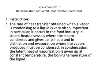
4.1 THE LUMPED CAPACITANCE METHOD A typical application in heat treatment is quenching where a metal or an alloy with initial temperature Ti is suddenly immersed in a liquid of lower temperature, T < Ti. This is shown in fig- chp5\fig5.1.pptx . If quenching begins at time t = 0, then given sufficient time, the temperature of the solid will decrease eventually to T . The heat transfer is due to convection on the surface. The assumption, here, is that the temperature of the solid is spatially uniform. This assumption, according to Fourier s law implies infinite k which is clearly impossible. But when 3
compared to the convective heat transfer resistance, it can approximately satisfy the above condition. Energy balance on the surface gives E E E E E st out g in + + = = + + E = = = = 0 in g After substitution dT E E = = = = hA ( T T ) Vc out st s dt Let Vc d T T , and this will give hA dt = = s 4
Separating the variables and integration gives i 0 s hA d Vc t = = dt where Evaluating the integrals will give Vc i = Ti T is the initial condition = = ln t or hA s i t T T hA = = = = exp s T T Vc i i The above equation gives the time required for the temperature to reach T or Temperature at a prescribed time t 5
The solution also indicates exponential decay as shown in fig-chp5\fig5.2.pptx . If we define t as the thermal time constant, which is an indicator of how fast the solid will respond to surrounding temperature change 1 = = = = ( Vc ) R C t t t hA s Where Rt = convection heat transfer resistance Ct = thermal capacitance (lumped) Increase in t (due to increase in Rt or Ct or both) 6
the solid will respond slowly. Total heat transfer up to some time t will be = = = = = = s dQ q dt hA ( T T dt ) hA dt s t t = = = = Q q dt hA dt s 0 0 Substitution of the solution gives = = t = = = = Q ( Vc ) 1 exp E E i out st t For quenching Q is positive and the solid experiences a decrease in energy. 7
5.2 VALIDITY OF THE LUMPED CAPACITANCE METHOD The previous method is the simplest and the most convenient method for the solution of transient problems. But it comes at a cost - the assumption made-infinite thermal conductivity Under what condition will this assumption hold? Consider the steady-state condition shown in fig- chp5\fig5.3.pptx . T <Ts,2<Ts,1. Under steady-state condition kA 2 , s 2 , s 1 , s = = ( T T ) hA ( T T ) L 8
Rearranging results in T T 2 , s 1 , s = = R L / kA hL = = = = cond , t Bi T T / 1 hA R k 2 , s conv , t Bi-Biot number-a dimensionless parameter which is a ratio of the two thermal resistances. Bi<<1: Rt,conv >> Rt,cond-equivalent to k Bi>>1: Rt,conv<< Rt,cond not good for lumped capacitance approach For transient processes, consider fig- chp5\fig5.4.pptx. The block is initially at Ti and experiences cooling when it is immersed in a fluid of T <Ti. 9
For Bi<<1 the temperature gradient in the block is small and T(x,t) T(t). For moderate to large values of Bi-temperature gradient is significant. The lumped capacitance method will hold true for hL Bi = = c 1 . 0 k Formula to be used for different geometries would require the definition of Lc, a characteristic length, as Lc = V/As 10
Plane wall: wall thickness L, Lc=(LhW)/2hW=L/2 Cylinder: radius ro, Lc=( ro2W)/2 roW=ro/2 Sphere: radius ro, [4/3( ro3)]/4 ro2 = ro/3 For conservative approach, Lc values Plane wall: same cylinder and sphere: ro Using Lc = V/As, the exponent of the transient equation may be expressed as (after some manipulation) hA t ht hL k t hL t = = = = = = . . s c c 2 c 2 c Vc cL k c L k L c 11
The above is a product of two dimensionless numbers t hA t = = Bi . Fo where Fo s 2 Vc L Fo is called Fourier number-dimensionless time. Substitution in the solution gives T T = = = = exp( Bi . Fo ) T T i i 12
Example 5.1 A thermocouple junction, which may be approximated as a sphere, is to be used for temperature measurement in a gas stream. The convection coefficient between the junction surface and the gas is h = 400 W/m2.K, and the junction thermophysical properties are k = 20 W/m.K, c = 400 J/kg.K, and =8500 kg/m3. Determine the junction diameter needed for the thermocouple to have a time constant of 1 s. If the junction is at 25oC and is placed in a gas stream that is at 200oC, how long will it take for the junction to reach 199oC? 13
Solution 1. As = D2 and V = D3/6 3 1 D = = x c t 2 h D 6 Substituting numerical values 6 c 6 h x 400 x 1 = = = = = = 4 D . 7 06 10 x m t 8500 x 400 With Lc = ro/3 4 r ( h ) 3 / 400 . 3 x 53 10 x = = = = = = 3 Bi . 2 35 10 x o k 3 x 20 Lumped capacitance method is an excellent approxim. 15
2. The time required for the junction to reach 199oC is 3 4 ( D c ) 6 / T T 8500 . 7 x 06 10 x x 400 25 200 = = = = t ln ln i 2 ( h D ) T T 6 x 400 199 200 = = t s 2 . 5 5 t 16
5.3 GENERAL LUMPED CAPACITANCE ANALYSIS Transient heat conduction can also be initiated by radiation; by a heat flux from a sheet of electrical heater attached to a surface, etc. fig-chp5\fig5.5.pptx depicts the influence of convection, radiation, an applied surface heat flux and internal energy generation. Applying energy conservation principle dT E + + + + = = ' ' s ' ' conv ' ' rad q A q ( q ) A Vc h , s g ) r , c ( s dt dT E + + ( h [ + + = = ' ' s 4 4 sur q A T T ) ( T T )] A Vc h , s g ) r , c ( s dt 17
The above is a non-linear, first order, non- homogeneous differential equation which can not be integrated to obtain an exact solution -requires approximate solution by numerical (finite difference) approach. Exact solution for simplified equation: (a)If no imposed heat flux or internal generation and convection is absent (vacuum) or negligible relative to radiation, the above equation simplifies to ( , = r s T A dt dT 4- 4 ) Vc T sur 18
Separating the variables and integrating dT dt Vc A t T = = r , s gives 4 sur 4 T T 0 T i 1 1 + + + + Vc T T T T T T = = + + t ln ln 2 tan tan sur sur i i 3 sur 4 A T T T T T T T r , s sur sur i sur sur The above will not give T explicitly and no solution for Tsur = 0 (deep space). However for Tsur = 0 in the above integral equation, it yields i r , s T T A 3 Vc 1 1 = = t 3 3 19
(b)For negligible radiation, and for = T-T , d/dt = dT/dt the equation reduces to a linear, first-order, non-homogeneous differential equation E g + + ' ' q A hA d h , s + + = = = = = = c , s a b 0 a b dt Vc Vc The above can be converted to a homogeneous equation by using ' b d + + = = ' ' results in a 0 a dt Separating variables and integrating from 0 to t gives the ) to ( i ' ' 20
solution as ' T T b ( ) a / = = = = exp( at ) exp( at ) ' T T b ( ) a / i i T T a / b = = + + exp( at ) 1 [ exp( at )] T T T T i i For steady state t , the equation reduces to (T-T )=(b/a) 21
Example 5.2 Consider the thermocouple and convection condition of example 5.1, but now allow for radiation exchange with the walls of a duct that encloses the gas stream. If the duct walls are at 400oC and the emissivity of the thermocouple bead is 0.9, calculate the steady-state temperature of the junction. Also, determine the time for the junction temperature to increase from initial condition of 25oC to a temperature that is within 1oC of its steady-state value. 22
Solution 1. Energy balance on the thermocouple ) T T ( [ sur E = = E 0 in out = = 4 4 ( h T T )] A 0 s Substituting numerical values gives T = 218.7oC 2. As this involves the transient part, the complete equation is out in E E = = E st dT 4 sur 4 [ + + = = ( h T T ) ( T T )] A Vc s dt Numerical solution for T = 217.7oC gives t = 4.9 s 24
5.4 SPATIAL EFFECTS For a one dimensional problem, the transient heat conduction equation can be determined from the general heat conduction equation as T 1 x 2 T 2 = = t The solution will require two boundary conditions and one initial condition given as (fig-chp5\fig5.4.pptx) IC: T(x,0) = Ti BC: (1) ( T/ x)@x=0= 0 (2) [-k( T/ x)@x=L] = h[T(L,t)-T ] 25
The solution will have a functional form of T=T(x, t, Ti, T , L, k, , h) (too many variables!) Non-dimensionalising the dependent variable T will reduce the number of variables as follows: Let =T-T , i = Ti T , dT = d Define *= / i then, dT = d = id * A dimensionless spatial coordinate is defined as x*=x/L dx = Ldx* and dimensionless time t*= ( t/L2) = Fo (Fourier No.), dt = (L2/ )dt* 26
Substituting the above in the transient conduction equation will give * 2 i ) / L ( x L i * 2 * * 1 = = = = or 2 * 2 2 * * 2 * t ( ) x t And the initial and the boundary conditions become 1 ) 0 , x ( = = = = = = * * * 0 * x * @ x 0 * = = * * Bi t , 1 ( ) * x * = = @ x 1 27
] where Bi = hL/k In dimensionless form, the functional dependence becomes * = f(x*, Fo, Bi) much simpler than the representation of function T. 5.5 PLANE WALL WITH CONVECTION This has an exact solution and also an approximate solution derived from the exact solution. 5.5.1 Exact Solution No attempt will be made to go through the steps of the exact solution. Referring to fig-chp5\fig5.6.pptx, a plane wall of thickness 2L with the assumption that 28
this thickness is much smaller than the width and height (allows one dimensional justification). For initial wall temperature, T(x,0) = Ti and suddenly immersed in a fluid of T , the exact solution is in series form and determined as Fo exp( C 1 n = = = = * 2 n * ) cos( x ) n n 4 + + sin = = C n n 2 sin( 2 ) n n 29
and the discrete values n, called eigenvalues are positive roots of the transcendental equation n tan n =Bi or tan n =Bi/ n The first few solutions for Bi=10 are given in the accompanying graph (fig-chp5\eigen1.pptx). Roots for different values of Bi are given in the handout. 5.5.2 Approximate Solutions For values of Fo>0.2, the infinite series solution can be approximated by the first term of the series only. This will give = = * 2 * C exp( Fo ) cos( x ) 1 1 1 30
At midplane (x*=0) fig-chp5\fig5.7.pptx T T 1 i = = * o 2 C exp( Fo ) o 1 T T This will give * = o* cos( 1x*) fig- chp5\fig5.8.pptx The above equation shows that the time dependence of the temperature at any location within the wall is the same as that of the midplane temperature. 5.5.3 Total Energy Transfer For a time interval from t=0 to any time t>0, energy conservation equation can be written as Ein Eout = Est 31
For heat transfer from the surface Ein = 0 and this gives Eout = - Est = Q Or Q = -[E(t) E(0)] = - c[T(x,t) Ti] dV To nondimensionalise, let Qo = cV(Ti T ) Qmaxat t The nondimensional expression will be fig- chp5\fig5.9.pptx = = Q o Q ) t , x ( T [ T ] dV 1 = = * 1 ( dV ) i T T V V i Use the approximate solution and with V= 2LWH, dV=(dx)WH=(dx*L)WH to get (x* 0 to 1) = = Q sin * o 1 1 Q 32 o 1
5.5.4 Additional Considerations The above solution is applicable to a plane wall, thickness L and insulated on one side (x* = 0). The foregoing results may be used to determine the transient response of a plane wall to a sudden change in surface temperature equivalent to h= which gives Bi = , and T replaced by Ts. 5.6 RADIAL SYSTEMS WITH CONVECTION 5.6.1 Infinite Cylinder For an infinite cylinder, the temperature change is in the radial direction only. This approximation can hold true for . 10 r / L o 33
5.6.1 Exact Solution In dimensionless form, the solution is given in series form as t 2 o = = = = * 2 n * C exp( Fo J ) ( r ) where Fo and n o n r = = n 1 2 J ( + + ) 2 1 = = C 1 n n 2 o J ( ) J ( ) n n n And the eigenvalues of n are positive roots of the transcendental equation ) ( J n 1 n = = Bi fig-chp5\eigen2.pptx J ( ) o n 34
where J1 and Jo are Bessel functions of the first kind of orders one and zero respecively. 5.6.2 Sphere For a sphere with radius ro, the exact solution is given by 1 ) Fo exp( C = = t = = = = * 2 n * sin( r ) where Fo n n * 2 o r r n 1 n [sin( 4 ) cos( )] = = C n n n n 2 sin( 2 ) n n 35
where the discreet values of n are the positive roots of the transcendental equation (fig-chp5\eigen3.pptx) 1 ncot n = Bi 5.6.2 Approximate Solutions For the infinite cylinder and sphere the series solution can be approximated by a single term for Fo>0.2 and the time dependence of the temperature at any location is the same as that of the centerline or centerpoint. Infinite Cylinder ( J ) Fo exp( C o 1 1 = = = = * 2 * r ) or 1 * * o * * o J ( r ) where is centerline T o 1 36
given by (@r = r* = 0) = = * o 2 C exp( Fo ) 1 1 fig-chp5\fig5.10.pptx , fig-chp5\fig5.11.pptx Sphere 1 = = * 2 * C exp( Fo ) sin( r ) or 1 1 1 * r 1 1 = = * * o * * o sin( r ) where is centerpo int T 1 * r 1 = = * o 2 C exp( Fo ) Given by fig-chp5\fig5.13.pptx , fig-chp5\fig5.14.pptx 1 1 37
5.6.3 Total Energy Transfer Using similar procedure as that of the plane wall, the heat transfers can be determined as: Infinite Cylinders 2 1 Q 1 o * o Q = = J ( ) 1 1 fig-chp5\fig5.12.pptx Sphere * o Q 3 = = 1 [sin( ) cos( )] 1 1 1 3 Q o 1 fig-chp5\fig5.15.pptx 38
5.6.4 Additional Considerations The above also gives the solution when the cylinder or sphere is subjected to a sudden change in surface temperature to Ts. Replace T by Ts which results due to infinite h value, hence infinite Bi. Example 5.3 A new process for treatment of a special material is to be evaluated. The material, a sphere of radius ro = 5 mm, is initially in equilibrium at 400oC in a furnace. It is suddenly removed from the furnace and subjected to a two-step cooling process. 39
Step 1 Cooling in air at 20oC for a period of time ta until the center temperature reaches a critical value, Ta(0,ta)=335oC. For this situation, the convective heat transfer coefficient is ha = 10 W/m2.K. After the sphere has reached this critical temperature, the second step is initiated. Step 2 Cooling in a well-stirred water bath at 20oC, with a convective heat transfer coefficient of hw = 6000W/m2.K. 40
= 3000 kg/m2, k=20 W/m.K, c=1000 J/kg.K and = 6.66 x 10⁻⁶ m2/s 1. Calculate the time ta required for step 1 of the cooling process to be completed. 2. Calculate the time tw required during step 2 of the process for the center of the sphere to cool from 335oC to 50oC. Solution 1. To check if lumped capacitance method can be used with Lc = ro/3, 005 . 0 x 10 k 3 h r = = = = = = 4 Bi . 8 33 10 x o o 3 x 20 41
Indeed the lumped capacitance method can be used. This will give T ln h 3 A h a a o s a Vc r c T = = = = t ln i o i a T T 3000 . 0 x 005 1000 x 400 20 = = = = ln 94 s 3 x 20 335 20 2. To check if the lumped capacitance method can be used 005 . 0 x 6000 k 3 h r = = = = = = Bi . 0 50 1 . 0 o o 3 x 20 Lumped capacitance method can not be used. A one term approximation can be used. 43
With the Biot number now defined as Bi=hwro/k=(6000x0.005)/20 = 1.50 The table gives C1 = 1.376 and 1 = 1.8 rad 1 Fo 1 1 = = * o 1 1 t , 0 ( T ) T = = = = ln ln x w 2 2 C C T T 1 1 i 1 1 50 20 = = ln x . 0 82 2 . 0 2 8 . 1 . 1 376 335 20 One term approximation is justifiable. r Fo t w = = = = 2 o 2 . 0 005 = = . 0 82 1 . 3 s 6 . 6 66 10 x 44
5.7 THE SEMI-INFINITE SOLID This is a geometry that is infinite in size in all but one direction having one surface only. The interior is well removed from the surface that it is unaffected by the surface condition. i.e. T(x ,t) = Ti A one dimensional transient equation can be used for such situation. Heat transfer near the surface of the earth or transient response of a thick slab are a few of the examples that can be mentioned. Three possible situations can exist on the surface as shown in fig-chp5\fig5.16.pptx . 45
The familiar equation will be used 2 T 1 x T = = = = . I . C ) 0 , x ( T T i 2 t Interior boundary condition T(x ,t) = Ti The above equation can be transformed into an ODE by using a function of the form = (x,t) that will result in T( ) instead of T(x,t). Transformation is done as follows: Use the transformation equation x/(4 t)1/2 46
to get the following derivatives x T dT 1 dT = = = = d d / 1 2 x ) t 4 ( 2 x T 2 d T d 1 dT 1 = = = = d d d / 1 2 / 1 2 x ) t ) t x 4 ( 4 ( 2 1 d T 2 = = 4 t d t t 2 T dT x dT dT = = = = = = d d d / 1 2 t ) t 4 ( t 2 47
Substitution gives 2 d T 2 dT = = 2 d d Boundary and initial conditions for case (1): For x = 0 = 0 T(0,t) T( =0) = Ts For x , and t=0 (both corresponding to ) T( ) = Ti The equation to be solved is d d dT dT d d d d dT = = = = 2 d 2 or dT d 48
Integration gives dT ln dT = = + + = = 2 ' 1 2 C or C exp( ) 1 d d Integrating a second time, we obtain = = + + 2 T C exp( u ) du C 1 2 0 u is a dummy variable. Applying the boundary condition T( =0) = Ts gives C2 = Ts The resulting equation will be 0 = = + + 2 T C exp( u ) du T 1 s 49
Applying the second boundary condition T( ) = Ti results in 0 = = + + 2 T C exp( u ) du T i 1 s Evaluating the definite integral gives ( 2 T T ) = = C i s 1 / 1 2 Hence the temperature distribution may be expressed as T T 2 / 1 s = = 2 2 ( / ) exp( u du ) erf T T 0 i s 50


/2hW=L/2")


For negligible radiation, and for θ = T-T∞ , dθ/dt =")


 fig-chp5\fig5.7.pptx")


")