Statistical Analysis of Laboratory Data Using limma-voom for RNA-Seq
Explore the application of limma-voom, a statistical method to analyze gene expression data from RNA-Seq experiments. Understand how this approach addresses the variance issue in RNA-Seq data by applying weights. Utilize bottomly data from inbred mouse strains to identify differentially expressed genes with limma-voom.

Uploaded on Oct 05, 2024 | 0 Views
Download Presentation

Please find below an Image/Link to download the presentation.
The content on the website is provided AS IS for your information and personal use only. It may not be sold, licensed, or shared on other websites without obtaining consent from the author. Download presentation by click this link. If you encounter any issues during the download, it is possible that the publisher has removed the file from their server.
E N D
Presentation Transcript
SPH 247 Statistical Analysis of Laboratory Data SPH 247 Statistical Analysis of Laboratory Data 1 May 5, 2015
limma-voom We have seen how limma can fit a linear model to each gene in microarray This is not limited to microarrays and can be used also with RNA-Seq data The main problem is that the linear models used in limma assume that the error variance is equal at all levels But in RNA-Seq, the variance rises with the mean Voom applies weights to address this problem. May 5, 2015 SPH 247 Statistical Analysis of Laboratory Data 2
Bottomly Data Two inbred mouse strains, C7BL6/6J (10 animals) and DBA/2J (11 animals) Gene expression in striatal neurons by RNA-Seq and expression arrays. 36,536 unique genes of which 11,870 had a count of at least 10 across the 21 samples. We can find differentially expressed genes with limma- voom April 28, 2015 SPH 247 Statistics for Laboratory Data 3
Data Files bottomly_count_table.txt 36536 rows (genes) plus one header row of column names 22 columns, 1 column of gene names, 10 C7BL6, 11 DBA2 gene SRX033480 SRX033488 SRX033481 SRX033489 1 ENSMUSG00000000001 369 744 287 769 2 ENSMUSG00000000003 0 0 0 0 3 ENSMUSG00000000028 0 1 0 1 4 ENSMUSG00000000031 0 0 0 0 5 ENSMUSG00000000037 0 1 1 5 May 5, 2015 SPH 247 Statistical Analysis of Laboratory Data 4
Data Files bottomly_phenodata.txt 21 rows, one per sample 5 columns sample.id num.tech.reps strain experiment.number lane.number 1 SRX033480 1 C57BL/6J 6 1 2 SRX033488 1 C57BL/6J 7 1 3 SRX033481 1 C57BL/6J 6 2 4 SRX033489 1 C57BL/6J 7 2 5 SRX033482 1 C57BL/6J 6 3 Three experiments (4, 6, 7), 7 lanes per experiment, C7BL6 in lanes 6, 7, 8 of experiment 4 C7BL6 in lanes 1, 2, 3, 5 of experiment 6 C7BL6 in lanes 1, 2, 3 of experiment 7 Two possible factors: strain (intended) experiment number (block?) May 5, 2015 SPH 247 Statistical Analysis of Laboratory Data 5
Input code source("input.bottomly.R") tmp <- read.table("bottomly_count_table.txt",header=T) count.data <- tmp[, -1] rownames(count.data) <- tmp[, 1] min.count <- 21 count.data <- count.data[which(rowSums(count.data) >= min.count), ] data2 <- read.table("bottomly_phenodata.txt", header=T) strain <- factor(as.character(data2$strain)) exp.num <- factor(as.character(data2$experiment.number)) 1) Reads count data from file 2) Eliminates gene names as a column, but adds them as row names 3) Filters data to eliminate genes with a mean count of less than one per sample (11175 of 36536 genes retained) 4) Reads characteristics of the sample 5) Creates variables for strain and experiment number May 5, 2015 SPH 247 Statistical Analysis of Laboratory Data 6
Analysis Code source("limma.analysis.R") require(limma) require(edgeR) dge <- DGEList(counts=count.data, genes=rownames(count.data), group=strain) dge <- calcNormFactors(dge) design1 <- model.matrix(~strain) v1 <- voom(dge, design1, plot =TRUE) fit1 <- lmFit(v1, design1) fit1 <- eBayes(fit1) 1) Creates dge object 2) Normalizes 3) Design matrix from strain only 4) Log transform and apply variance weights with voom 5) Fits linear models to each gene 6) Shrinks variances May 5, 2015 SPH 247 Statistical Analysis of Laboratory Data 7
May 5, 2015 SPH 247 Statistical Analysis of Laboratory Data 8
Results > names(fit1) [1] "coefficients" "stdev.unscaled" "sigma" "df.residual" [5] "cov.coefficients" "pivot" "genes" "Amean" [9] "method" "design" "df.prior" "s2.prior" [13] "var.prior" "proportion" "s2.post" "t" [17] "df.total" "p.value" "lods" "F" [21] "F.p.value" > colnames(fit1$p.value) [1] "(Intercept)" "strainDBA/2J > hist(fit1$p.value[,2]) > sum(fit1$p.value[,2] < 1e-4) [1] 385 > sum(p.adjust(fit1$p.value[,2],"fdr") < 0.05) [1] 1011 May 5, 2015 SPH 247 Statistical Analysis of Laboratory Data 9
May 5, 2015 SPH 247 Statistical Analysis of Laboratory Data 10
Exercise Edit code so that exp.num is fit as well as strain. Compare the number of FDR significant genes What is the overlap? design2 <- model.matrix(~exp.num+strain) The p.value matrix will have four columns instead of 2. Note that the blocking variables should be first in the formula if any kind of anova will be done. May 5, 2015 SPH 247 Statistical Analysis of Laboratory Data 11