Optimal Power Flow in Power System Operation and Control
The lecture covers Optimal Power Flow (OPF) and Linear Programming in power systems, discussing economic dispatch, contingency analysis, and constraints such as power balance, voltage setpoints, and transmission limits. Various components and constraints of OPF, as well as example solution methods, are explored in detail.

Download Presentation

Please find below an Image/Link to download the presentation.
The content on the website is provided AS IS for your information and personal use only. It may not be sold, licensed, or shared on other websites without obtaining consent from the author. Download presentation by click this link. If you encounter any issues during the download, it is possible that the publisher has removed the file from their server.
E N D
Presentation Transcript
ECEN 460 Power System Operation and Control Lecture 17: Optimal Power Flow, Linear Programming Prof. Tom Overbye Dept. of Electrical and Computer Engineering Texas A&M University overbye@tamu.edu
Announcements Finish reading Chapter 6 Homework 6 is due today Design project is assigned today, due on Dec 2; details are on the website Lab 8 (on OPF and LMP markets) is next week in WEB 115; no lab week of Nov 13 Exam 2 is during class on November 14 Final exam is as per the TAMU schedule, Wednesday Dec 13 from 8 to 10am 1
Design Project System Eagle Island Electric Company (IEC) 1.013 pu 12% Robin 1.021 pu 43% 1.020 pu 43% 42% Flamingo Pheasant 0.991 pu 83 Mvar 95 MW 23 Mvar 505 MW System Losses: 42.12 MW 110 MW 20 Mvar 87 MW 19 Mvar 1.000 pu 300 MW 12% 200 MW 60 Mvar 9% 4% 1.010 pu Canary 1.009 pu 160 MW 35 Mvar 9% 75 MW 15 Mvar 198 MW 35 Mvar 150 MW 50 Mvar 1.015 pu 56 Mvar 32% 34% 0.993 pu 0.995 pu Dove 112 MW 40 Mvar 78 Mvar Woodpecker 11% 10% Rook 32% 10% 9% 5% 1.019 pu 1.010 pu 0.995 pu 115 MW 25 Mvar 1.019 pu Cardinal 1.010 pu 20% Parrot 23% 22% 1.011 pu 48% 0.990 pu 75 Mvar 268 MW 128 Mvar Turkey 16% 132 MW 10 Mvar 30% Sparrow 1.008 pu 5% 21% 14% 32% 1.003 pu 1.009 pu Bluebird 0.993 pu 56% 380 MW 13% 17% 28% 17% 175 MW 30 Mvar Ostrich 1.008 pu 0.991 pu 21% 132 MW 15 Mvar 1.015 pu Mallard 27% 23% 150 MW 39 Mvar 51 Mvar 3% 29% Owl NewWind 0.994 pu 170 MW 24 Mvar 1.010 pu 0.990 pu 72 Mvar 29% Hawk 70 Mvar 130 MW 45 Mvar Piper 37% 10% 0.000 pu 2% 165 MW 30 Mvar 35% Oriole 0.986 pu Kiwi 7% 1.015 pu 39% 0.997 pu 0.991 pu 22% slack 12% Crow 680 MW 0.985 pu 36% 140 MW 32 Mvar 10% 0 MW 176 MW 15 Mvar 4% 17% 23% 128 MW 28 Mvar 135 MW 10 Mvar 49% 0.985 pu Heron 150 MW 52 Mvar Lark 0.994 pu 46% Finch 0.995 pu 6% 22% 161 MW 21 Mvar Condor 47% 140 MW 20 Mvar 53% 1.025 pu 46% Peacock 1.001 pu 1.008 pu Hen 800 MW 9% 1120 MW 88 MW 11 Mvar 48% 48% 1.020 pu 2
Optimal Power Flow (OPF) Next we ll consider OPF and SCOPF OPF functionally combines the power flow with economic dispatch SCOPF adds in contingency analysis In both minimize a cost function, such as operating cost, taking into account realistic equality and inequality constraints Equality constraints bus real and reactive power balance generator voltage setpoints area MW interchange 3
OPF, contd Inequality constraints transmission line/transformer/interface flow limits generator MW limits generator reactive power capability curves bus voltage magnitudes (not yet implemented in Simulator OPF) Available Controls generator MW outputs transformer taps and phase angles reactive power controls 4
Two Example OPF Solution Methods Non-linear approach using Newton s method handles marginal losses well, but is relatively slow and has problems determining binding constraints Generation costs (and other costs) represented by quadratic or cubic functions Linear Programming fast and efficient in determining binding constraints, but can have difficulty with marginal losses. used in PowerWorld Simulator Generation costs (and other costs) represented by piecewise linear functions 5
LP OPF Solution Method Solution iterates between solving a full ac power flow solution enforces real/reactive power balance at each bus enforces generator reactive limits system controls are assumed fixed takes into account non-linearities solving a primal LP changes system controls to enforce linearized constraints while minimizing cost 6
Two Bus with Unconstrained Line With no overloads the OPF matches the economic dispatch Transmission line is not overloaded Total Hourly Cost : Area Lambda : 13.01 8459 $/hr Bus B Bus A 13.01 $/MWh 13.01 $/MWh 300.0 MW MW 300.0 MW MW 197.0 MW AGC ON MW 403.0 MW AGC ON MW Marginal cost of supplying power to each bus (locational marginal costs) 7
Two Bus with Constrained Line Total Hourly Cost : Area Lambda : 13.26 9513 $/hr Bus B Bus A 13.43 $/MWh 13.08 $/MWh 380.0 MW MW 300.0 MW MW 260.9 MW AGC ON MW 419.1 MW AGC ON MW With the line loaded to its limit, additional load at Bus A must be supplied locally, causing the marginal costs to diverge. 8
Three Bus (B3) Example Consider a three bus case (bus 1 is system slack), with all buses connected through 0.1 pu reactance lines, each with a 100 MVA limit Let the generator marginal costs be Bus 1: 10 $ / MWhr; Range = 0 to 400 MW Bus 2: 12 $ / MWhr; Range = 0 to 400 MW Bus 3: 20 $ / MWhr; Range = 0 to 400 MW Assume a single 180 MW load at bus 2 9
B3 with Line Limits NOT Enforced 60 MW 60 MW Bus 2 Bus 1 10.00 $/MWh 0.0 MW 10.00 $/MWh 120 MW 180.0 MW 120% 0 MW Line between Bus 1and Bus 3 is over-loaded; all buses have the same marginal cost 60 MW 120% 120 MW Total Cost 1800 $/hr 60 MW 10.00 $/MWh Bus 3 180 MW 0 MW 10
B3 with Line Limits Enforced 20 MW 20 MW Bus 2 Bus 1 10.00 $/MWh 60.0 MW 12.00 $/MWh 100 MW 120.0 MW 100% 0 MW 80 MW LP OPF changes generation to remove violation. Bus marginal costs are now different. 100% 100 MW Total Cost 1920 $/hr 80 MW 14.00 $/MWh Bus 3 180 MW 0 MW 11
Verify Bus 3 Marginal Cost 19 MW 19 MW Bus 2 Bus 1 10.00 $/MWh 62.0 MW 12.00 $/MWh 100 MW 119.0 MW 100% 81% 0 MW 81 MW One additional MW of load at bus 3 raised total cost by 14 $/hr, as G2 went up by 2 MW and G1 went down by 1MW 100% 81% 100 MW Total Cost 1934 $/hr 81 MW 14.00 $/MWh Bus 3 181 MW 0 MW 12
Why is bus 3 LMP = $14 /MWh All lines have equal impedance. Power flow in a simple network distributes inversely to impedance of path. For bus 1 to supply 1 MW to bus 3, 2/3 MW would take direct path from 1 to 3, while 1/3 MW would loop around from 1 to 2 to 3. Likewise, for bus 2 to supply 1 MW to bus 3, 2/3MW would go from 2 to 3, while 1/3 MW would go from 2 to 1to 3. 13
Why is bus 3 LMP $ 14 / MWh, contd With the line from 1 to 3 limited, no additional power flows are allowed on it. To supply 1 more MW to bus 3 we need Pg1 + Pg2 = 1 MW 2/3 Pg1 + 1/3 Pg2 = 0; (no more flow on 1-3) Solving requires we up Pg2 by 2 MW and drop Pg1 by 1 MW -- a net increase of $14. 14
Both lines into Bus 3 Congested 0 MW 0 MW Bus 2 Bus 1 10.00 $/MWh 100.0 MW 12.00 $/MWh 100 MW 100.0 MW 100% 100% 0 MW For bus 3 loads above 200 MW, the load must be supplied locally. Then what if the bus 3 generator opens? 100 MW 100% 100% 100 MW Total Cost 2280 $/hr 100 MW 20.00 $/MWh Bus 3 204 MW 4 MW 15
Quick Coverage of Linear Programming LP is probably the most widely used mathematical programming technique It is used to solve linear, constrained minimization (or maximization) problems in which the objective function and the constraints can be written as linear functions 16
Example Problem 1 Assume that you operate a lumber mill which makes both construction-grade and finish-grade boards from the logs it receives. Suppose it takes 2 hours to rough-saw and 3 hours to plane each 1000 board feet of construction-grade boards. Finish- grade boards take 2 hours to rough-saw and 5 hours to plane for each 1000 board feet. Assume that the saw is available 8 hours per day, while the plane is available 15 hours per day. If the profit per 1000 board feet is $100 for construction-grade and $120 for finish-grade, how many board feet of each should you make per day to maximize your profit? 17
Problem 1 Setup Let x =amount of cg, x = amount of fg Maximize 100 s.t. 2 2 3 5 , x x 1 2 + 120 x x x + + x 1 2 8 15 x x 1 2 1 2 0 1 2 Notice that all of the equations are linear, but they are inequality, as opposed to equality, constraints; we are seeking to determine the values of x1 and x2 18
Example Problem 2 A nutritionist is planning a meal with 2 foods: A and B. Each ounce of A costs $ 0.20, and has 2 units of fat, 1 of carbohydrate, and 4 of protein. Each ounce of B costs $0.25, and has 3 units of fat, 3 of carbohydrate, and 3 of protein. Provide the least cost meal which has no more than 20 units of fat, but with at least 12 units of carbohydrates and 24 units of protein. 19
Problem 2 Setup Let x =ounces of A, x = ounces of B Minimize 0.20 s.t. 2 3 3 4 3 , x x Again all of the equations are linear, but they are inequality, as opposed to equality, constraints; we are again seeking to determine the values of x1 and x2; notice there are also more constraints then solution variables 1 2 + 0.25 x x + x 1 2 20 x 1 + 2 15 x x 1 x 2 x + 24 1 2 0 1 2 20
Three Bus Case Formulation For the earlier three bus system given the initial condition of an overloaded transmission line, minimize the cost of generation ( PG1, PG2, PG3) such that the change in generation is zero, and the flow on the line between buses 1 and 3 is not violating its limit 1800 $/hr 60 MW 60 MW Bus 2 Bus 1 10.00 $/MWh 0.0 MW 10.00 $/MWh 120 MW 180.0 MW 120% 0 MW 60 MW 120% 120 MW Total Cost 60 MW 10.00 $/MWh Bus 3 180 MW 0 MW 21
Three Bus Case Problem Setup Let x = P , x = P , x = P Minimize 10 2 s.t. 3 enforcing limits on , , 1 G1 2 G2 x 3 G3 + + 12 1 3 20 x x 1 2 3 + 20 x x Line flow constraint 1 2 Power balance constraint + + = 0 x x x 1 2 3 x x x 1 2 3 22
LP Standard Form The standard form of the LP problem is Minimize s.t. where n-dimensional column vector n-dimensional row vector m-dimensional column vector m n matrix For the LP problem usually n The previous examples were not in this form! cx Ax x x c b A Maximum problems can be treated as minimizing the negative = 0 b = = = = m 23
Replacing Inequality Constraints with Equality Constraints The LP standard form does not allow inequality constraints Inequality constraints can be replaced with equality constraints through the introduction of slack variables, each of which must be greater than or equal to zero + = = with with 0 0 b b y y b b y y i i i i i i i i 24
Lumber Mill Example with Slack Variables Let the slack variables be x3 and x4, so Minimize -(100 s.t. 2 3 , x x x x + Minimize the negative 120 + + ) = = x x 1 2 5 , 2 + + 8 15 x x x x x x 1 2 3 1 2 , 4 0 1 2 3 4 25
LP Definitions x A vector is said to be basic if 1. 2. At most m components of are non-zero if there as less than m non-zeros the is called degenerate = x = x = Ax b x x x B = x x A A A Define (with basic) and AB is called the basis matrix B B N N x ( ) B 1 = A A b x A b A x With so B N B N B N N 26
LP Definitions x A vector is said to be feasible if 1. 2. A basic solution is not necessarily feasible, and a feasible solution is not necessarily basic. We'll also assume is full rank, so always has a solution = 0 Ax x b = A Ax b An m by n matrix (with m < n) is rank m if there are m linearly independent columns 27
Fundamental LP Theorem Given an LP in standard form with A of rank m then If there is a feasible solution, there is a basic feasible solution If there is an optimal, feasible solution, then there is an optimal, basic feasible solution Note, there could be a LARGE number of basic, feasible solutions Simplex algorithm determines the optimal, basic feasible solution 28
Simplex Algorithm The key is to move intelligently from one basic feasible solution to another, with the goal of continually decreasing the cost function The algorithm does this by determining the best variable to bring into the basis; this requires that another variable exit the basis, while retaining a basic, feasible solution 29
At the Solution At the solution we have m non-zero elements of x, xB, and n-m zero elements of x, xN ( ) 1 = x A b N N A x We also have B B 1 = c A And we define B B The elements of tell the incremental cost of enforcing each constraint (just like in economic dispatch) 30
Lumber Mill Example Solution + Minimize -(100 s.t. 2 3 , The solution is 120 + + ) = = x x 1 2 5 , = 2 + + 8 15 x x x x x x 1 2 3 An initial basic feasible solution is 0, 0, x x x = = 1 2 , 4 = = 8, 15 x 1 2 3 4 0 = x x x x x 1 2 3 2.5, 4 = = 1.5, 0, 0 x x x 1 2 3 4 1 2 3 2 5 35 10 = Then = 100 120 Economic interpretation of is the profit is increased by 35 for every hour we up the first constraint (the saw) and by 10 for every hour we up the second constraint (plane) 31
LP Sensitivity Matrix (A Matrix) for Three Bus Example 32
Example 6_23 Optimal Power Flow In the example the load is gradually increased 33
Locational Marginal Costs (LMPs) In an OPF solution, the bus LMPs tell the marginal cost of supplying electricity to that bus The term congestion is used to indicate when there are elements (such as transmission lines or transformers) that are at their limits; that is, the constraint is binding Without losses and without congestion, all the LMPs would be the same Congestion or losses causes unequal LMPs LMPs are often shown using color contours; a challenge is to select the right color range! 34
Example 6_23 Optimal Power Flow with Load Scale = 1.72 35
Example 6_23 Optimal Power Flow with Load Scale = 1.72 LP Sensitivity Matrix (A Matrix) The first row is the power balance constraint, while the second row is the line flow constraint. The matrix only has the line flows that are being enforced. 36
Example 6_23 Optimal Power Flow with Load Scale = 1.82 This situation is infeasible, at least with available controls. There is a solution because the OPF is allowing one of the constraints to violate (at high cost) 143 MW 54 Mvar 80 MW 80 MW 124 MW 124 MW A A 57% MVA 57% MVA 1.05 pu 0.99 pu 1.00 pu 3 4 1 16.82 $/MWh 20.74 $/MWh 22.07 $/MWh 213 AGC ON MW 133 MW 64 MW 268 MW 71 Mvar 42 MW slack A A 280 AGC ON MW 89% MVA A 58% MVA 100% MVA A 48% MVA 64 MW 56 MW 176 MW 133 MW A 42 MW 100% MVA 1.04 pu 0.95 pu 176 MW 15.91 $/MWh 1101.78 $/MWh 5 2 220 AGC ON MW 71 MW 36 Mvar 231.9 71.3 Mvar MW 11297.88 $/h Total Hourly Cost: Load Scalar: 1.82 713.4 MW Total Area Load: 235.47 $/MWh Marginal Cost ($/MWh): 37


")


 Example")


 for")

")