Principles of Data Arrangement and Presentation for Effective Analysis

Effective data arrangement and presentation are crucial for engaging readers, maintaining conciseness, and enabling quick insights and conclusions. Methods such as textual, tabular, and graphical presentations aid in statistical analysis. Learn about the importance of organizing data from lowest to highest, stem-and-leaf plots, and various chart types like bar graphs and pie charts.

Download Presentation

Please find below an Image/Link to download the presentation.
The content on the website is provided AS IS for your information and personal use only. It may not be sold, licensed, or shared on other websites without obtaining consent from the author. Download presentation by click this link. If you encounter any issues during the download, it is possible that the publisher has removed the file from their server.
E N D
Presentation Transcript
DATA ARRANGEMENT AND PRESENTATION formation of tables and charts DATA ARRANGEMENT AND PRESENTATION formation of tables and charts
Presentation of data Principles: Data should be arranged in such a way that it will arouse interest in reader. The data should be made sufficiently concise without losing important details. The data should presented in simple form to enable the reader to form quick impressions and to draw some conclusion, directly or indirectly. Should facilitate further statistical analysis . It should define the problem and suggest its solution
Methods of presentation of data The first step in statistical analysis is to present data in an easy way to be understood. There are three ways for data presentation. These are: Textual Method Tabulation Graphical Method
Presentation of data Textual Method Rearrangement from lowest to highest Stem-and- leaf plot Textual Method Tabular Method Frequency distribution table (FDT) Relative FDT Tabular Method Graphical Bar Chart Graphical Method Method Histogram Cumulative FDT Frequency Polygon Pie Chart
Textual Presentation of Data If we are present the performance of our section in the Statistics test. The following are the test scores of our class: 34 42 20 50 17 9 34 43 50 18 35 43 50 23 23 35 37 38 38 39 39 38 38 39 24 29 25 26 28 27 44 44 49 48 46 45 45 46 45 46
Solution: First, arrange the data in order for you to identify the important characteristics. This can be done in two ways: rearranging from lowest to highest or using the stem-and-leaf plot. Below is the rearrangement of data from lowest to highest: 9 23 28 35 38 43 45 48 17 24 29 37 39 43 45 49 18 25 34 38 39 44 46 50 20 26 34 38 39 44 46 50 23 27 35 38 42 45 46 50
Stem-and-leaf Plot Data rearrangement is done by making use of the stem-and-leaf plot. Stem-and-leaf Plot is a table which sorts data according to a certain pattern. separating a number into two parts. In a two- digit number, the stem consists of the first digit, and the leaf consists of the second digit. While in a three-digit number, the stem consists of the first two digits, and the leaf consists of the last digit. In a one-digit number, the stem is zero. It involves
Below is the stem-and-leaf plot of the ungrouped data given in the example. Stem 0 1 2 3 4 5 Leaves 9 7,8 0,3,3,4,5,6,7,8,9 4,4,5,5,7,8,8,8,8,9,9,9 2,3,3,4,4,5,5,5,6,6,6,8,9 0,0,0 Utilizing the stem-and-leaf plot, we can readily see the order of the data. Thus, we can say that the top ten got scores 50, 50, 50, 49, 48, 46, 46, 46,45, and 45 and the ten lowest scores are 9, 17, 18, 20, 23,23,24,25,26, and 27.
TABULAR METHOD TABULAR METHOD
Rules and guidelines for tabular presentation Table must be numbered Brief and self explanatory title must be given to each table. The heading of columns and rows must be clear, sufficient, concise and fully defined. The data must be presented according to size of importance, chronologically, alphabetically or geographically Table should not be too large. Figures needing comparison should be placed as close as possible
The classes should be fully defined, should not lead to any ambiguity. The classes should be exhaustive i.e. should include all the given values. The classes should be mutually exclusive and non overlapping. The classes should be of equal width or class interval should be same Open ended classes should be avoided as far as possible. The number of classes should be neither too large nor too small. Can be 10-20 classes. Formula for number of classes(C): C=1+3.322 log(n), where n is total number of observation in data.
Frequency Distribution Table A frequency distribution table is a table which shows the data arranged into different classes(or categories) and the number of cases(or frequencies) which fall into each class. Grouped Data vs. Ungrouped Data Ungrouped data is the data you first gather from an experiment or study. The data is raw form that is, it s not sorted into categories and classified. Grouped data is data that has been bundled together in categories.Histograms and frequency tables can be used to show this type of data.
Sample of a Frequency Distribution Table for Ungrouped Data
Relative Frequency Table Relative frequency = class frequency ( ) sum of all frequencies( )
Cumulative Frequency Table Cumulative Frequency Table
Exercise: The following data shows the ages of 50 cancer patients admitted in Shaukat Khanum Memorial Hospital, Lahore: 48 29 31 32 54 33 44 36 38 31 46 30 20 44 47 39 42 35 33 47 31 35 34 42 41 42 43 35 32 35 43 36 37 45 46 41 25 27 26 40 38 41 44 47 45 45 52 43 44 43 Make a frequency distribution table. Find out class boundaries , mid points, relative frequency and cumulative relative frequency from a given data.
GRAPHICAL METHOD GRAPHICAL METHOD
Charts and diagrams Charts and diagrams Graphic presentations used to illustrate and clarify information. Tables are essential in presentation of scientific data and diagrams are complementary to summarize these tables in an easy, attractive and simple way.
The Charts should be: Simple Easy to understand Save a lot of words Self explanatory Has a clear title indicating its content Fully labeled The y axis (vertical) is usually used for frequency
Various charts and diagrams Bar Chart Histogram Frequency polygon Cumulative frequency curve Scatter Chart Line Chart Pie diagram
Bar Chart Widely used, easy to prepare tool for comparing categories of mutually exclusive discrete data. Different categories are indicated on one axis and frequency of data in each category on another axis. Length of the bar indicate the magnitude of the frequency of the character to be compared. The width of the bar and the gaps between the bars should be equal throughout. The bars may be vertical or horizontal. 3 types of bar diagram: o Simple o Multiple or compound o Component or proportional
Simple Bar Chart Exports of Pakistan (in US $ million) Year Exports 1948 138 1951 406 1961 378 1971 683 1981 2958 1991 6168 2001 9202 2005 14410
Multiple Compound Bar Chart 1. Multiple bar chart is an extension of simple bar chart. 2. Grouped bars are used to represent related sets of data. For example, imports and exports of a country together are shown in multiple bar chart. 3. Each bar in a group is shaded or coloured differently for the sake of distinction Imports Exports Rs. (billion) 68.15 76.71 89.78 90.95 92.43 111.38 Years Rs. (billion) 34.44 37.33 37.98 49.59 63.35 78.44 1982-83 1983-84 1984-85 1985-86 1986-87 1987-88
Component or proportional bar chart Subdivision of a single bar to indicate the composition of the total divided into sections according to their relative proportion. For example two communities are compared in their proportion of energy obtained from various food stuff, each bar represents energy intake by one community, the height of the bar is 100, it is divided horizontally into 3 components (Protein, Fat and carbohydrate) of diet, each component is represented by different color or shape.
Histogram Used for Quantitative, Continuous Variables. It is used to present variables which have no gaps e.g age, weight, height, blood pressure, blood sugar etc. It consist of a series of blocks. The class intervals are given along horizontal axis and the frequency along the vertical axis.
Frequency Polygon Derived from a histogram by connecting the mid points of the tops of the rectangles in the histogram. The line connecting the centers of histogram rectangles is called frequency polygon. We can draw polygon without rectangles so we will get simpler form of line graph. A special type of frequency polygon is the Normal Distribution Curve.
Sex Frequency polygon Age MP M F (12% (10% ) (30% ) (25% ) (15% ) (20% ) 20- 25 ) Males Females % (36% 30- 35 ) 40 35 40- (8%) 45 30 (16% 50- 55 25 ) 20 60- 70 (8%) 65 15 10 5 0 Age 25 35 45 55 65 Figure (2): Distribution of 45 patients at (place) , in (time) by age and sex
Frequency curve 9 Female Male 8 7 6 Frequency 5 4 3 2 1 0 20- 30- 40- 50- 60-69 Age in years
Cumulative frequency diagram or O give An ogive is a graph that represents cumulative frequencies or cumulative relative frequencies of a data set. The cumulative frequency is plotted on the y-axis against the data which is on the x-axis for un-grouped data. When dealing with grouped data, the Ogive is formed by plotting the cumulative frequency against the upper boundary of the class.
Cumulative frequency for ungrouped data Age (years) 10 11 12 13 14 15 16 17 Cumulative Frequency 5 5+10 = 15 15+27 = 42 42+18 = 60 60+6 = 66 66+16 = 82 82+38 = 120 120+9 = 129 Frequency 5 10 27 18 6 16 38 9
Constructing an Ogive Here is the Frequency Distribution for the attendance (in thousands) at Super Bowl Data for games I to XXXVI (1 to 36): Class Limits Class Freq. Relative Frequency Cumulative Frequency Cumulative Relative Frequency Boundaries 62-69 70-77 78-85 86-93 94-101 102-109 61.5-69.5 69.5-77.5 77.5-85.5 85.5-93.5 93.5-101.5 101.5-109.5 3 .08 .53 .22 .03 .06 .08 19 8 1 2 3 Notice the two extra columns.
Cumulative Values Cumulative Frequencies and Cumulative Relative Frequencies represent running totals for the two columns which precede them. Below is a complete frequency distribution.
Step 1: Draw a Cumulative Relative Frequency Histogram.
Percentiles A percentile is a certain percentage of a set of data. Percentiles are used to observe how many of a given set of data fall within a certain percentage range; for example; a thirtieth percentile indicates data that lies the 13% mark of the entire data set. Calculating Percentiles Percentile as Pmwhere m represents the percentile we're finding, for example for the tenth percentile,m} would be 10. Given that the total number of elements in the data set is N
Quartiles The term quartile is derived from the word quarter which means one fourth of something. Thus a quartile is a certain fourth of a data set. When you arrange a date set increasing order from the lowest to the highest, then you divide this data into groups of four, you end up with quartiles. There are three quartiles that are studied in statistics. First Quartile (Q1)-------(1 4) 25th percentile (n + 1) 4 Second Quartile (Q2) ---(2 4) 50th percentile 2(n + 1) 4 Third Quartile (Q3)------(3 4) 75th percentile 3(n + 1) 4
Age (years) 10 11 12 13 14 15 16 17 Cumulative Frequency 5 15 42 60 66 82 120 129 Frequency 5 10 27 18 6 16 38 9 Interquartile Range The interquartile range is the difference between the third quartile and the first quartile.
Scatter/ dot diagram Also called as Correlation diagram ,it is useful to represent the relationship between two numeric measurements, each observation being represented by a point corresponding to its value on each axis. In negative correlation, the points will be scattered in downward direction, meaning that the relation between the two studied measurements is controversial i.e. if one measure increases the other decreases While in positive correlation, the points will be scattered in upward direction.


")