Understanding Propensity Score Methods for Reducing Confounding in Studies
This content discusses the use of propensity score methods to address confounding in observational studies, comparing randomized control trials (RCTs) with observational studies, explaining the potential outcome framework, average treatment effects, and common assumptions made in these methods to reduce bias and draw valid conclusions in research.
- Propensity score methods
- Observational studies
- Confounding
- Average treatment effects
- Randomized control trials
Download Presentation

Please find below an Image/Link to download the presentation.
The content on the website is provided AS IS for your information and personal use only. It may not be sold, licensed, or shared on other websites without obtaining consent from the author. Download presentation by click this link. If you encounter any issues during the download, it is possible that the publisher has removed the file from their server.
E N D
Presentation Transcript
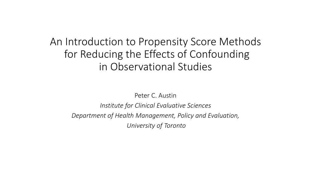
An Introduction to Propensity Score Methods for Reducing the Effects of Confounding in Observational Studies Peter C. Austin Institute for Clinical Evaluative Sciences Department of Health Management, Policy and Evaluation, University of Toronto
Overview potential outcomes framework causal treatment effects Randomized Control Trials (RCTs) Observational Studies Propensity score Methods of applying propensity scores
Potential Outcome Framework and Average Treatment Effects Two possible treatments Active Treatment (T=1) and Control Treatment (T=0) Active Treatment (T=1) and Control Treatment (T=0) Pair of potential outcomes Y Yi i (0) and Y (0) and Yi i (1) (1) Actual Observed Outcome Y Yi i = = T Ti i Y Yi i (1) + (1 (1) + (1 - - T Ti i) Y ) Yi i (0) (0) Treatment Effect for each patient Yi(1) - Yi(0) Average Treatment Effect (ATE) E[Yi (1) Yi (0)]
RCTs vs Observational Studies In RCTs, treatment assignment is done by randomization No systematic differences between the Treated and Controlled X T P(x) = P(x|T=1) = P(x|T=0) ATE can be defined as ATE = E[Yi (1) Yi (0)]=E[Y(1)|T=1]-E[Y(0)|T=0] ATE can be derived using the data Simply plug in the values of the treated samples to controlled samples and vice versa.
RCTs vs Observational Studies (Cont.) In observational studies, we do not use randomization to allocate units to treatment and control groups Systematic differences between the Treated and Controlled P(x) P(x|T=1) P(x|T=0) And also for ATE we have ATE = E[Yi (1) Yi (0)] E[Y(1)|T=1] - E[Y(0)|T=0] Deriving the ATE from the data is impossible without making a lot of assumptions
Most Common Assumptions No unmeasured confounders: treatment assignment (T) is independent of the potential outcomes (Y(0) and Y(1)) conditional on the observed baseline covariates (X). (Y(1), Y(0)) T | X Common support: every subject has a nonzero probability to receive either treatment 0 < P(T=1|X) < 1
Propensity Score The probability of treatment assignment conditional on observed baseline covariates ei = Pr(Ti = 1|Xi) 1-ei = Pr(Ti = 0|Xi) A balancing score: conditional on the propensity score, the distribution of measured baseline covariates is similar between treated and untreated subjects. Subjects with the same propensity score, the distribution of observed baseline covariates will be the same between the treated and untreated subjects. Xi T|ei
Propensity Score Based Methods Methods of using propensity score to evaluate the Average Treatment Effect (ATE) We will discuss three methods: Propensity Score Matching Inverse Probability of Treatment Weighting Using the Propensity Score All of these methods assume that both of the assumptions hold: (Y(1), Y(0)) T | X 0 < P(T=1|X) < 1
Propensity Score Matching Forming matched sets of treated and untreated subjects who share a similar value of the propensity score. Most common way: one-to-one or pair matching, in which pairs of treated and untreated subjects are formed, such that matched subjects have similar values of the propensity score. Once a matched sample has been formed, the treatment effect can be estimated by directly comparing outcomes between treated and untreated subjects in the matched sample ATE is the difference between the mean outcome for treated subjects and the mean outcome for untreated subjects in the matched sample.
Propensity Score Matching (Cont.) Matching with/without replacement: matching without replacement: Each untreated subject is included in at most one matched set. matching with replacement: A given untreated subject can be included in more than one matched set. Greedy/Optimal matching: Greedy matching: the nearest untreated subject is selected for matching to the given treated subject. Optimal matching: matches are formed so as to minimize the total within-pair difference of the propensity score.
Inverse Probability of Treatment Weighting Using the Propensity Score Uses weights based on the propensity score to create a synthetic sample in which the distribution of measured baseline covariates is independent of treatment assignment.
Inverse Probability of Treatment Weighting Using the Propensity Score A subject s weight is equal to the inverse of the probability of receiving the treatment that the subject actually received wi=Ti ei+1 Ti 1 ei Using the weight, ATE can be calculated as ATE = 1 ???? ?? 1 (1 ??)?? 1 ?? ? ? ? ?=1 ? ?=1 The weights may be inaccurate or unstable for subjects with a very low probability of receiving the treatment received
