Introduction to Econometrics and Machine Learning

Econometrics and machine learning intersect in decision-making scenarios where causal and counterfactual questions arise. This talk explores the relationship between the two fields, highlighting the identification of causal quantities and the flexible estimation techniques employed. Examples demonstrate how machine learning methods can be used to estimate effects such as price elasticity of demand, considering potential confounding variables along the way.

Download Presentation

Please find below an Image/Link to download the presentation.
The content on the website is provided AS IS for your information and personal use only. It may not be sold, licensed, or shared on other websites without obtaining consent from the author. Download presentation by click this link. If you encounter any issues during the download, it is possible that the publisher has removed the file from their server.
E N D
Presentation Transcript
Econometrics and Machine Learning Vasilis Syrgkanis Microsoft Research New England
Econometrics and Machine Learning Machine learning infiltrating decision making Most decision-making questions are causal/counterfactual At odds with ML power: prediction vs counterfactual prediction Econometrics -> ML: recipes for identification of causal quantities ML -> Econometrics: flexible non-parametric estimation
What is Machine Learning For this talk: 2 min ?? ? ? ? is some hypothesis space: random forests, neural nets, high- dimensional linear functions, boosted forests More generally generalization bounds with respect to some loss Several times implies mean squared error consistency for ?[? ?]
Example 1: Estimating Effect of Price on Demand
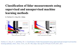
Example: Estimating Price Elasticity of Demand Goal: Estimate elasticity, the effect of a change in price on demand log(demand) ? = ?0 ? + ? noise log(demand) elasticity log(price) log(price) Conclusion: Increasing price increases demand! Problem: Demand increases in winter and price anticipates demand
Example: Estimating Price Elasticity of Demand Goal: Estimate elasticity, the effect of a change in price on demand log(demand) ? = ?0 ? + ?0 ? + ? season indicator log(demand) noise elasticity log(price) log(price) Idea: Introduce confounder (the season) into regression
Example: Estimating Price Elasticity of Demand Goal: Estimate elasticity, the effect of a change in price on demand log(demand) ? = ?0 ? + ?0 ? + ? season indicator log(demand) noise elasticity log(price) log(price) Problem: What if there are 100s or 1000s of potential confounders?
Example: Estimating Price Elasticity of Demand Problem: What if there are 100s or 1000s of potential confounders? Time of day, day of week, month, purchase and browsing history, other product prices, demographics, weather, One Option: Estimate effect of all potential confounders really well ? = ?0 ? + ?0? + ? log(demand) elasticity log(price) effect of potential confounders noise If nuisance function ?0 is estimable at ? ? 1/2 rate then so is ?0 Problem: Accurate nuisance estimates often unachievable when ?0 is non-parametric or linear and high-dimensional
Double ML for Treatment Effect Inference Double Machine Learning [Chernozhukov, Chetverikov, Demirer, Duflo, Hansen, Newey 2017] 1. Regress ? ?, learn ?[?|?] 2. Regress ? ?, learn ?[?|?] (mean treatment policy) 3. Linear regression on residuals: ? ? ? ? ? ? ? ?] 1 ? ? Coefficient in final regression is treatment effect ? Guarantees Neyman orthogonal estimator of ?0 robust to first-order errors in nuisance estimates; yields ?-consistent and asymptotically normal estimate of ?0 Nuisance estimates can be fitted by arbitrary ML methods, subject to achieving RMSE consistency at the slow rate of ? ? 1/4 2 ?? ? ? ? ? ? ? ? ? min ?
Some Remarks In order to estimate a causal effect and at a fast rate, we had to estimate other nuisance functions The current theorem applied to the estimation of a constant treatment effect ?; for personalized decisions we want a heterogeneous treatment effect ?(?) We want to build a complex ML model for ?(?)
Triple ML for Treatment Effect Inference Triple ML [Chernozhukov et al 2017a,b], [Nie, Wager, 2017] 1. Regress ? ?, learn q X = ?[?|?] 2. Regress ? ?, learn p X = ?[?|?] (mean treatment policy) 3. Minimize residual square loss: 1 ? ? ?? ? ?? ? ?? (?? ? ??)2 min ? Nie, Wager: Reproducing Kernel Hilbert spaces Error in final regression is of the same order as if we knew the nuisance functions Chernozhukov, Nekipelov, Semenova, S: Sparse linear Athey, Wager; Oprescu, S, Wu: Random Forests
Walkthrough Example 2: Binary Treatments
Binary Treatment Effects Binary Treatment: ?? {0,1} Pr ??= ? ??= ? = ??(?) Simply taking an average of the treated and untreated is biased due to confoundeness A model-heavy approach Regress ? ?,?,?, learn htX = ?[?|? = ?,?] ? =1 ? ? 1?? 0??
Binary Treatment Effects Binary Treatment: ?? {0,1} Pr ??= ? ??= ? = ??(?) Simply taking an average of the treated and untreated is biased due to confoundeness A non-parametric approach: Inverse Propensity Weighting =?? 1{??= ?} ? =1 ? ? ? ??, IPS ???? ??,??? (1) ??,??? (0)
Binary Treatment Effects Binary Treatment: ?? {0,1} Pr ??= ? ??= ? = ??(?) Simply taking an average of the treated and untreated is biased due to confoundeness Doubly Robust ?? ??? 1{??= ?} ???? (1) ??,DR ? ??, DR = ??? + ? =1 (0) ? ??, DR ?
Triple ML for Treatment Effect Inference Triple ML: Binary Treatment [Foster, Syrgkanis, 2019], [Oprescu, Wu, Syrgkanis, 2018] 1. Regress ? ?,?, learn htX = ?[?|? = ?,?] 2. Regress ? ?, learn p?X = ?[? = ?|?] (prob of treatment) 3. Doubly Robust Target: ?? ??? 1{??= ?} ???? ? ??, DR = ??? + (1) ??,DR (0)~ ?: 4. Regress??, DR 2 1 ? (1) ??,DR (0) ? ?? ??, DR min ? ?
Optimal Treatment Policy ? ??, DR If we were to follow a treatment policy: ?:? {0,1} ???? =1 ? are good estimates of the counterfactual outcomes 1 0 ? ? ??, DR + 1 ? ? ??, DR ? Is a good estimate of the value of the policy ? Maximize over space of policies: 1 ? 1 0 min ? ???? = min ? ?? ??, DR ??, DR ? ? [Athey, Wager, 17], [Zhou, Athey, Wager, 18]: VC classes [Foster, S. 19]: Rademacher complexity, entropy integral [Demirer, S., Chernozhukov, Lewis 19]: Continuous actions
Technical Vignette: Orthogonal Statistical Learning [Foster, S., COLT 2019 (best paper)]
Orthogonal Statistical Learning Target model ? is the minimizer of an expected loss function ?0= argmin ???;?0 ? Which also depends on nuisance functions ?0whose true value we don t know and need to estimate Oracle Excess Risk. given ? samples, find an estimate ? such that ?? ?;?0 ???0;?0 ?? Examples Pricing: ???;? = ? ?? ? ?? ? ?? (?? ? ??)2 2 1 0 Binary: ???;? = ? ??, DR ??,DR ? ?? 1 0 Policy: ???;? = E ? ?? ??, DR ??, DR
Machine Learning and Generalization Machine learning is good at achieving excess risk for known losses For any loss function ??? , find ? such that: ?? ? ???0 ?? Most ML theory addresses such questions (generalization bounds) Excess risk has meaningful problem-specific interpretations 2 ? ? ?0? For square losses it implies mean squared error: ? For policy learning it is a bound on the regret of a policy Can we reduce our problem to what ML is good at?
Side Advantages of Excess Risk Fewer Assumptions Does not require stringent assumptions on identification of parameters of model (e.g. full rank co-variance of features, restricted eigenvalue conditions) Allow for Mis-Specification Convergence to best within class model w.r.t. some distance metric Can be easily combined with analysis of mis-specification bias
Meta-Algorithm Split samples in half Stage 1. Estimate ? on first half, with estimation error ? ?0 ??? Stage 2. Estimate ? on second half in a plugin manner: use any algorithm that guarantees ?? ?; ? ???0; ? ??? When does this algorithm achieve good oracle excess risk? ?? ?;?0 ???0;?0 ???
Neyman Orthogonality Directional derivative: ?????;? [??] =? ????? + ? ??;? A loss ???;? is Neyman orthogonal if: ???????0;?0[??,??] = 0 Intuition: Small perturbation of nuisance ? around its true value, do not change the gradient information of the loss with respect to target Example: pricing ? ?? ? ?? ? ?? (?? ? ??)2 ????? ;?0 ??,?? = 2? ?? ? ?? ? ?? ?? ? ?? ??????? ;?0[??,??] = 2? ?? ? ?? ?? ? ?? = 0 ???? ????
Main Theorem 1 If loss is orthogonal, strongly convex in ? and smooth, ? first-order optimal ??? ??? + ???4 Assumptions. Let ??= ? ? , ??= ? ?0 1. Strongly Convex: ?????,? ??,?? ? ?? 2. Smooth: ?? 4 2 ? ?? 2???,?0 ??,?? ? ?? 2 2 2????? ,? ??,??,?? ? ?? ?? 3. First-order Optimality: ????? ,?0 ? ? 0 ??
Proof Sketch 1 Strongly Convex at ?: ?? ?, ? ??? ; ? ????? ; ? ? ? ? Neyman Orthogonal and smooth: ????? ; ? ????? ;?0 + ?? 2 2????? ,? ??,??,??
Proof Sketch 1 Strongly Convex at ?: ?? ?, ? ??? ; ? ????? ; ? ? ? ? Neyman Orthogonal and smooth: ????? ; ? ????? ;?0 + ? ?? ?? 2 2
Proof Sketch 1 Strongly Convex at ?: ?? ?, ? ??? ; ? ????? ; ? ? ? ? Neyman Orthogonal and smooth: ????? ; ? ????? ;?0 + ???4+ ? ? ? ? 2 2
Proof Sketch 1 Strongly Convex at ?: 2 ?? ?, ? ??? ; ? ????? ; ? ? ? ? Neyman Orthogonal and smooth: ????? ; ? ~ ????? ;?0 + ???4+ ? ? ? ? 2 First order optimality of ? : ? ? 2~ 1 ?????? ;?0 + ??? + ???4 ??? + ???4 0 Smoothness: ?? ?,?0 ??? ;?0 ????? ;?0 +? 2 ~ ??? + ???4 ? ? 2
Unobserved Confounders & Instrumental Variables
Unobserved Confoundedness ? = ?0(?) ? + ?0? + ? outcome heterogeneous effect treatment effect of potential confounders noise ? is not observed One solution: Instrumental variables Variables ? that affect ? but does not directly affect ? ? = ?0(?) ? ? = ? ? + ? + ?
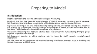
Example: Estimating Price Elasticity of Demand Goal: Estimate elasticity, the effect of a change in price on demand Instrument: weather in brasil affects production cost of coffee and hence price of coffee but does not directly affect the demand in US log(demand) log(demand) Good weather Good weather Avg demand in bad weather Bad weather Bad weather log(price) log(price) Avg price in bad weather
More generally: 2SLS ML 1. Regress ? ? to learn ? [?|?] 2. Linear regression ? ?[?|?] to learn ? ML log(demand) log(demand) Good weather Good weather Avg demand in bad weather Bad weather Bad weather log(price) log(price) Avg price in bad weather Requires the demand function (counterfactual function) to be linear in price (treatment)
More generally: 2SLS ML 1. Regress ? ?,? to learn ? [?|?,?] 2. Linear regression ? ? ? ?,? ,? to learn ?(?) ML log(demand) log(demand) Good weather Good weather Avg demand in bad weather Bad weather Bad weather log(price) log(price) Avg price in bad weather Requires the demand function (counterfactual function) to be linear in price (treatment)
Intent-to-Treat A/B Test: TripAdvisor Example Value of membership. What is the value of becoming a member and which visitors are high-value? Treatment: becoming a member Outcome: number of visits, revenue spend Features: features of the user, e.g. past web history, geolocation, platform How to measure? We cannot run an A/B test where we force half of the users to become members We cannot measure the revenue of members vs non-members (self-selection bias=unobserved confounders) Solution. We can run a recommendation A/B test!
Effect of Membership on TripAdvisor [S., Lei, Oprescu, Hei, Battocchi, Lewis, 19] A/B Test: For random half of 4million users, easier sign-up flow was enabled Easier sign-up incentivizes membership Recommendation has an effect on whether you become a member No direct effect on downstream engagement A/B test can be used as an instrument
IV Estimation for Intent-to-Treat A/B Test [S., Lei, Oprescu, Hei, Battocchi, Lewis, 19] outcome No recommendation: ? = 0 outcome Avg response with no rec Gave recommendation: ? = 1 treatment treatment Prob of treatment when Z=1 T=0 T=1
Discontinuous Policy ML T=0 Income T=1 Treatment effect ML SAT Score Threshold for getting into college
Synthetic Controls Local Revenue effect UK ML Canada ML South US time Built a new Azure data center in Canada [Abadie et al, 03, 10, 15, 16], [Synthetic Learner, Bradic, Viviano, 19]
Differences-in-Differences Local ML Revenue effect time Built a new Azure data center in Canada [Synthetic Diff-in-Diff, Arkhangelsky et al, 18]
Take-Aways Econometrics interested in causality ML is good at prediction/correlation Often extracting causal quantities can reduce to set of prediction tasks Econometrics provides recipes for identifying causal quantities ML can be used for prediction sub-tasks of these recipes [Double/Debiased ML, Chernozhukov et al, 18], [ML Estimation of Hetero Effects with Instruments, S. et al, 19], [Synthetic Learner, Bradic, Viviano, 19], [Synthetic Diff-in-Diff, Arkhangelsky et al, 18] ML can be used for automated detection/estimation of heterogeneity in the causal quantity of interest as function of observables [Generalized/Causal Forests, Tibshirani, Athey, Wager, 19], [Quasi-Oracle Estimation of Hetero Effects, Nie, Wager, 17], [ML Estimation of Hetero Effects with Instruments, S. et al, 19] Very rich and interesting theoretical research on Propagation of estimation errors [Orthogonal Statistical Learning, Foster, S., COLT19] Valid confidence intervals/hypothesis testing [Causal Forests, Athey, Wager, 19], [Orthogonal Random Forests, Oprescu, S, Wu, 19], [Double/Debiased ML, Chernozhukov et al, 18]
A Python Library Go to our GitHub repo: https://github.com/microsoft/econml Check out our documentation: https://econml.azurewebsites.net/ Install EconML: pip install econml
EconML Unified API Outcome (Y) Treatment (T) Features (X) Treatment Effect (X) Test Features (Xtest) EconML Estimator Controls (W) Instruments (Z)
EconML Unified API Each estimator has a `fit` and `effect` function with the same signature. Example usage: from econml.dml import DMLCateEstimator est = DMLCateEstimator( ) est.fit(Y, T, X, W) #function signature: fit(Y, T, X, W=None, Z=None) est.effect(X, T0, T1) #function signature: effect(X, T0=0, T1=1) For detailed information, see the docs econml.azurewebsites.net.
Linear Treatment Effect Orange Juice Elasticity Linear parametric form Polynomial Treatment Effect Polynomial parametric form
Git Repo: Git Repo: https://github.com/Microsoft/EconML Documentation: Documentation: https://econml.azurewebsites.net Learn more about the ALICE project: Learn more about the ALICE project: https:// https://aka.ms/alice Thank you! Greg Lewis Keith Battocchi Miruna Oprescu Paul Oka Vasilis Syrgkanis Maggie Hei
What is the effect of ? on achievable rate? One might worry that the best achievable rate for ?? ?; ? ???0; ? ??? Might be worse than that for: ?? ?;?0 ???0;?0 ??? If target model space is convex, then the impact is at most constants (rate analysis solely uses the first order condition) If target model space is non-convex, then tighter rates could potentially be achievable under ?0because proofs depend on well- specifiedness of the model. However, orthogonality can save us again!
Empirical Risk Minimization Suppose the second stage algorithm is plug-in ERM ? = argmin? ?? ? ? ,? ? ,? If loss is strongly convex in ? ? , then fast rates are captured by local Rademacher complexity 1 ? ???,? = ? sup ?? ? ?? ?: ?2 ? ? Let ???? ?0 = {? ? ?0:? ,? [0,1]} Let critical radius, solution to inequality: ???,???? ?0 ?2
ERM and Local Rademacher Without nuisance functions, ERM achieves: 2 ??? ~ ?? Proof invokes first order optimality condition (convexity or well- specifiedness) We extend proof to plugin ERM under orthogonality: ??? ~ ?? 2+ ???4