Integration Approaches of Propensity Scores in Epidemiologic Research

Propensity scores play a crucial role in epidemiologic research by helping address confounding variables. They can be integrated into analysis in various ways, such as through regression adjustment, stratification, matching, and inverse probability of treatment weights. Each integration approach has its strengths and limitations, affecting the estimation of treatment effects. Regression adjustment with propensity scores can reduce bias in estimating treatment effects, offering advantages over traditional regression models. Understanding these integration methods is essential for effectively utilizing propensity scores in research.
- Propensity Scores
- Epidemiologic Research
- Integration Approaches
- Regression Adjustment
- Treatment Effects

Download Presentation

Please find below an Image/Link to download the presentation.
The content on the website is provided AS IS for your information and personal use only. It may not be sold, licensed, or shared on other websites without obtaining consent from the author. Download presentation by click this link. If you encounter any issues during the download, it is possible that the publisher has removed the file from their server.
E N D
Presentation Transcript
Propensity Score Analysis in Epidemiologic Research - PART II: PS Integration OSCTR BERD WORKSHOP May 25th, 2022 Tabitha Garwe, PhD MPH Associate Professor Director, Surgical Outcomes Research Associate Director BERD Co-Director BERD Clinical Epidemiology Unit 1
Strengths and Limitations Use of propensity scores as effective as variables selected for model Unlike a well-designed RCT - benefit does not extend to unmeasured covariates If some confounders are unobserved, individuals that have the same observed covariates might not have the same probability of being assigned to the treated group. Sensitivity analysis Generally requires a large sample size Significant imbalances of certain covariates may be unavoidable despite a well constructed propensity score Simpler to determine whether the propensity score model has been adequately specified than to assess whether the regression model relating treatment assignment and baseline covariates to the outcome has been correctly specified balance diagnostics One can explicitly examine the degree of overlap in the distribution of baseline covariates between the two treatment groups. Increased flexibility when outcomes are rare and treatment is common
Integration Approaches Propensity scores can be integrated into an analysis in a number of ways Most common Raw score regression adjustment Stratification Matching Inverse probability of treatment weights (IPTW) Creates weights that are appropriate for estimating the ATE and ATT Allows for population based inferences, but results can be sensitive to estimated weights (in particular when outlier observations exist)
Regression Adjustment Score as an additional covariate (i.e., in addition to the treatment variable) can be included directly as a probability ranging from 0 to 1 or can be multiplied by a fixed value (e.g., 1,000) serves as a composite confounder regression analysis may include only the treatment variable and the propensity score as covariates, or additional important covariates. Roseman, 1994 - if the response surfaces in the treatment and control groups are parallel and either linear or non-linear, then the regression adjustment using the propensity scores reduces the bias in the estimate of the treatment effect i.e. no interaction between ps and treatment group
Regression Adjustment Is there any gain in using the propensity score rather than performing a regression adjustment with all of the covariates used to estimate the propensity score included in the model? Should give the same results The main advantage of the two-step process one can first fit a very complicated propensity score model with interactions and higher order terms and not be concerned with over-parameterizing this model. A smaller model may allow the investigator to perform diagnostic checks on the fit of the model more reliably Recall restrictions on the number of covariates that may be included in a given model
Regression Adjustment In general, regression adjustment should be performed with caution. Rubin (1979) showed that regression adjustment may in fact increase the expected squared bias if the covariance matrices (of independent variables) in the treated and untreated groups are unequal Another difficulty arises when the variance in the treated and untreated groups are very different (that is, the untreated group variance is much larger than the treated groups variance). consider using propensity score methods for matching or sub-classification, rather than using covariance adjustment
Stratification Propensity score is a scalar summary of all the observed background covariates Stratification on it alone can balance the distributions of the covariates in the treated and control groups Quintiles generally used Cochran(1968) - creating five strata removes 90 per cent of the bias due to the stratifying variable or covariate Rosenbaum & Rubin (1984) - found that using five strata based on the estimated propensity score was able to substantially reduce the bias
Stratification There must be adequate overlap in propensity scores between treatment groups to produce valid estimates for treatment effects. Estimate the treatment effects separately within each quintile defined by the propensity score and then combine the quintile estimates into an overall estimate subjects in each quintile of propensity score are compared with a univariate test for treatment effect results can be combined across strata (e.g., the Mantel-Haenszel method for averaging ORs across strata) - Breslow- Day Test Has been suggested to exclude strata where one of the treatment groups is inadequately represented, e.g., <10% (Ioannidis et al., 2001) Stratified regression Weighted regression can estimate the ATT if you weight by the stratum-specific number of treated units can estimate the ATE if you weight by the stratum-specific number of units (treated and control units combined)
Matching Generally viewed as the most statistically efficient method of incorporating propensity scores, but requires a large sample size and eliminates unmatched subjects Treated and untreated subjects share a similar value of the propensity score Can estimate ATT Pair matching (1 to 1) most common Estimating treatment effect after matching, analyze as matched sample or not? some debate around this Within the matched sample, the treated and untreated subjects should be regarded as independent [Schafer and Kang (2008)] When using a matched estimator, the variance should be calculated using a method appropriate for paired experiments [Imbens (2004)] Simulation studies - variance estimators that account for matching more accurately reflected the sampling variability of the estimated treatment effect (Austin 2009) Propensity score matching can be combined with additional matching on prognostic factors or regression adjustment (Imbens, 2004; Rubin & Thomas, 2000). 9
Matching Matching with replacement Allows a given untreated subject to be included in more than one matched set Variance estimation must account for the fact that the same untreated subject may be in multiple matched sets (Hill & Reiter, 2006). Matching without replacement (most common) Selected untreated subject no longer available for subsequent treated subjects Optimal Matching matches are formed so as to minimize the total within-pair difference of the propensity score selects all matches simultaneously and without replacement to minimize the total absolute difference in propensity score across all matches. Fixed ratio matching, requested by the METHOD=OPTIMAL option (in SAS PROC PSMATCH) matches a fixed number of control units to each treated unit Variable ratio matching, requested by the METHOD=VARRATIO option (in SAS PROC PSMATCH) matches one or more control units to each treated unit Full matching (METHOD=FULL) involves forming matched sets consisting of either one treated subject and at least one untreated subject or one untreated subject and at least one treated subject. Improved bias reduction obtained when matching with a variable number of controls compared to matching with a fixed number of controls [Ming and Rosenbaum (2000)] 10
MATCHING Greedy Matching Treated subject is first selected at random Untreated subject whose propensity score is closest to that of this randomly selected treated subject is chosen for matching; sequential matching Greedy - the nearest untreated subject is selected for matching, even if that untreated subject would better serve as a match for a subsequent treated subject. Criteria for closest (for both optimal and greedy) Nearest neighbor matching nearest - no restrictions are placed upon the maximum acceptable difference Nearest neighbor matching within a specified caliper distance - further restriction that the absolute difference in the propensity scores of matched subjects must be below some prespecified threshold (the caliper distance). 11
Matching Rosenbaum and Rubin outline three techniques for constructing a matched sample which use the propensity score (Rosenbaum & Rubin, 1985) Nearest available matching on the estimated propensity score Mahalanobis metric matching including the propensity score Nearest available Mahalanobis metric matching within calipers defined by the propensity score best technique among the three Rosenbaum and Rubin suggest using the logit of the estimated propensity score to match distribution is often approximately normal. Calipers of width equal to 0.2 of the pooled standard deviation of the logits of the propensity score will eliminate approximately 99% of the bias due to the measured confounders.
Software Considerations Proc PSMATCH (SAS) Can be used for prospensity score stratification, matching and weighting PSMATCH2 (Stata) Match it (R Software) 13
SAS PROC PSMATCH https://support.sas.com/documentation/onlinedoc/stat/142/psmatch.pdf 14
REGION (For matching, stratification and weighting) Specifies an interval region of propensity scores (or equivalently, logits of propensity scores) that determines which observations are used in stratification and matching. REGION=ALLOBS selects all available observations REGION=TREATED selects observations whose propensity scores lie in the region of propensity scores for observations in the treated group. REGION=Common Support (CS) selects observations whose propensity scores (or equivalently, logits of propensity scores) lie in the region of common support for the treated and control groups largest interval that contains propensity scores (or logits of propensity scores) for subjects in both groups. The lower endpoint of the region is the larger of the minimum propensity scores (or logits of propensity scores) for the two groups. The upper endpoint is the smaller of the maximum propensity scores (or logits of propensity scores) for the two groups. 15
Inverse probability of treatment weights (IPTW) Creates weights that are appropriate for estimating the ATE and ATT Uses weights based on the propensity score to create a synthetic sample in which the distribution of measured baseline covariates is independent of treatment assignment. similar to the use of survey sampling weights A subject s weight is equal to the inverse of the probability of receiving the treatment that the subject actually received. Regression models can be weighted by the inverse probability of treatment to estimate causal effects of treatments. In this context, IPTW is part of a larger family of causal methods known as marginal structural models (Hernan, Brumback, & Robins, 2000, 2002). Variance estimation must account for the weighted nature of the synthetic sample Weights may be inaccurate or unstable for subjects with a very low or very high probability of receiving the treatment received. Stabilizing weights recommended 18
IPTW-ATE Where pj=propensity score Stabilized IPTW-ATE ATT Weighting ATT weighting (also called weighting by odds) computes the weight for the jth observation with propensity score pj as https://support.sas.com/documentation/onlinedoc/stat/142/psmatch.pdf 19
Very low or very high probability of receiving the treatment received Garwe et al., J Trauma. 2011;70: 120 129) 20


")