Understanding Profit Maximization and Revenue Concepts in Economics
Explore the concepts of profit maximization, revenue generation, and marginal analysis in economics. Learn how to define profit, calculate total revenue and cost, and understand marginal revenue. Discover the significance of marginal value of product and its impact on business decision-making.

Uploaded on Oct 02, 2024 | 0 Views
Download Presentation

Please find below an Image/Link to download the presentation.
The content on the website is provided AS IS for your information and personal use only. It may not be sold, licensed, or shared on other websites without obtaining consent from the author. Download presentation by click this link. If you encounter any issues during the download, it is possible that the publisher has removed the file from their server.
E N D
Presentation Transcript
Profit Maximization Beattie, Taylor, and Watts Sections: 3.1b-c, 3.2c, 4.2-4.3, 5.2a-d 1
Agenda Generalized Profit Maximization Profit Maximization with One Input and One Output Profit Maximization with Two Inputs and One Output Profit Maximization with One Input and Two Outputs 2
Defining Profit Profit can be generally defined as total revenue minus total cost. Total revenue is the summation of the revenue from each enterprise. The revenue from one enterprise is defined as price multiplied by quantity. Total cost is the summation of all fixed and variable cost. 3
Defining Profit Cont. Short-run profit ( ) can be defined mathematically as the following: TC TR = n m = = = ( , ,..., , , ,..., ) y y y x x x p y w x TFC 1 2 1 2 n m i i j j 1 1 i j = ( , ,..., ) y f x ( x , x 1 1 11 12 1 m = ,..., ) y f x x x 2 2 21 22 2 m = ( , ,..., ) y f x x x 2 1 2 n n x n nm x = + + + x x 1 11 21 1 n = + + + x x x x 2 12 22 2 n = + + + x x x x 4 1 2 m m m nm
Revenue In a perfectly competitive market revenue from a particular enterprise can be defined as p*y. When the producer can have an effect on price, then price becomes a function of output, which can be represented as p(y)*y. 5
Marginal Revenue Marginal Revenue (MR) is defined as the change in revenue due to a change in output. In a perfectly competitive world, marginal revenue equals average revenue which equals price. = TR py dTR = = MR p dy 6
Marginal Revenue Cont. When the market is not perfectly competitive, then MR can be represented as the following: = ( ) * TR p y y dTR = = + ( ' ) * ( ) MR p y y p y dy ( ' ) * p y ( y = + ( ) 1 MR p y ) p y 1 1 = + = + ( ) 1 ( ) 1 MR p y p y d d 7
Marginal Value Of Product Marginal Value of Product (MVP) is defined as the change in revenue due to a change in the input. To find MVP, you need to substitute the production function y=f(x) into the TR function. = ( ) TR y py = ( ) ( ) TR x pf x ( ) dTR x = = = ( ' ) MVP pf x pMPP dx 8
Cost Side of Profit Maximization Marginal Cost (MC) and Marginal Input Cost (MIC) can be derived from the cost side of the profit function. Marginal cost is defined as the change in cost due to a change in output. From the cost minimization problem, it was shown the different forms that marginal cost could take. Marginal Input Cost is the change in cost due to a change in the input. MIC is equal to the price of the input. 9
Standard Profit Maximization Model n m = Max = ,..., 1 for p y w x TFC i i j j = . . . w r t 1 1 i j for ,..., 1 y i n i = = , ; ,..., 1 x y i n x ( j m ij = ( ,..., ) f x , x 1 1 11 12 1 m = ,..., ) y f x x x 2 2 21 22 2 m = ( , ,..., ) y f x x x 2 1 2 n n x n nm x = + + + x x 1 11 21 1 n = + + + x x x x 2 12 22 2 n = + + + x x x x 1 2 m m m nm 10
Profit Maximization with One Input and One Output Assume that we have one variable input (x) which costs w. Assume that the general production function can be represented as y = f(x). Max x py wx TFC , y = subject to : ( ) y f x 11
Examining Results of Profit Maximization with One Input and One Output = + ( , , ) ( ( ) ) x y py wx TFC f x y d = + = ( ' ) 0 w f x dx d = = 0 p dy d = = ( ) 0 f x y dy w ( ' = and = p ) f x w ( ' = p ) f ) x = ( ' pf x w = pMPP w = MVP MIC 12
Notes on Profit Maximization By solving the profit maximization problem, we get the optimum decision rule where MVP=MIC. With minor manipulation we can transform the result from the previous slide using the production function into the other form of the optimum decision MR = MC. 13
Notes on Profit Maximization Cont. There are two primary ways to solve the profit maximization problem. Solve the constrained profit max problem w.r.t. x and y. Transform the constrained profit max problem into an unconstrained problem by substituting the production function or its inverse into the profit max problem and solve w.r.t. to the appropriate variable. 14
Solving the Profit Maximization Problem W.R.T. Inputs Assume that we have one variable input (x) which costs w. Assume that the general production function can be represented as y = f(x). ( ) Max x pf x wx TFC 15
Solving the Profit Maximization Problem W.R.T. Inputs Cont. = ( ) ( ) x pf x wx d = = ( ' ) 0 pf x w dx = ( ' ) pf x w = w pMPP w = MPP p 16
Solving the Profit Maximization Problem W.R.T. Outputs Assume that we have one variable input (x) which costs w. Assume that the general production function can be represented as y = f(x) with an output price of p. 1 ( ) Max y py wf y TFC 17
Solving the Profit Maximization Problem W.R.T. Outputs Cont. = 1 ( ) ( ) y py wf y TFC d w = = 0 p dx MPP w = p MPP w = MPP p 18
Profit Max Example 1 Suppose that you would like to maximize profits given the following information: Output Price = 10 Input Price = 200 TFC = 100 y=f(x)=50x-x2 19
Profit Max Example 1: Lagrangean = = 2 10 200 100 s.t. ( ) 50 Max x y x y f x x x , y d = + 2 ( , , ) 10 200 100 50 ( ) x y y x x x y = + = 200 50 ( 2 ) 0 x dx d = = 10 0 dy d = = 2 50 0 x x y d Solution w ill be done in class. 20
Profit Max Example 1: Unconstrained W.R.T. Input ( ) 2 10 50 200 100 Max x x x x ( ) d = 2 ( ) 10 50 200 100 x x x x = = 10 50 ( 2 ) 200 0 x dx = 10 50 ( x 2 ) 200 x = 50 ( x 2 = ) 20 x 2 = 30 15 f = = 15 ( ) 525 y = 2150 21
Profit Max Example 1: Solving Using MIC=MVP = w 200 = p 10 = = 2 2 ( ) = 10 w 50 ( = dTR ) 500 10 TR x x x x x 200 MIC = = 500 20 MVP x dx = MVP MIC = 500 x 20 200 x x = 300 20 = 15 22
Profit Max Example 1: Solving Using MPP=w/p = w 200 = p 10 = = 2 ( ) dy 50 y f x x x = = 50 2 MPP x dx w = MPP p 200 = 50 2 x 10 x = 2 = 30 x 15 23
Profit Max Example 1: Unconstrained W.R.T. Output = = 2 ( ) 50 y f x x x = = 1 ( ) 25 625 x f y y ( ) max y 10 200 25 625 100 y y ( ) = ( ) 10 200 25 625 100 y y y 1 200 d = = 10 0 2 dy 625 y 100 = 10 625 y 1 1 = 10 625 y = 10 625 y = 100 625 - y = y 525 = = 1 - x f (525) 15 24
Profit Max Example 1: Solving Using MC=MR = = 2 ( ) 50 y f x x x w = = 1 ( ) 25 TFC 625 = x f y y = = 200 , 10 + , 100 p = p = + = ( ) 200 ( 25 625 ) 100 5100 200 625 TC y wx TFC y y = = 10 MR 1 200 100 dTC = = ) 1 = 0 * ( MC 2 dy 625 625 y y = MR MC 100 = 10 625 y 1 1 = 10 625 y = 10 625 y = 100 625 - y = y 525 25
Question: How would you find the loss in profit ( ) if you were a revenue maximizer instead a profit maximizer? Loss = -Max- Revenue-Max 26
Note on Calculating Profit at Revenue Max Profit at revenue max can be found by calculating profit at the revenue maximizing point, i.e., find the input level where MPP=0, calculate the output for this level of input, and then use these values to calculate profit 27
Graph of Profit and Production 3000 2000 1000 Production Profit 0 0 5 10 15 20 25 30 35 -1000 -2000 28
Graph of Profit and Total Revenue 7000 6000 5000 4000 Total Revenue Profit 3000 2000 1000 0 0 5 10 15 20 25 30 35 29
Graph of Marginal Revenue and Marginal Cost 50 40 30 Marginal Revenue Marginal Cost 20 10 0 0 100 200 300 400 500 600 700 30
Graph of Marginal Value of Product and Marginal Input Cost 31
Profit Max Example 2 Suppose that you would like to maximize profits given the following information: Output Price = 20 Input Price = 200 TFC=100 y=f(x)=50x-x2 32
Profit Max Example 2: Lagrangean = = 2 20 200 100 s.t. ( ) 50 Max x y x y f x x x , y d = + 2 ( , , ) 20 200 100 50 ( ) x y y x x x y = + = 200 50 ( 2 ) 0 x dx d = = 20 0 dy d = = 2 50 0 x x y d Solution w ill be done in class. 33
Profit Max Example 2: Unconstrained W.R.T. Input ( ( 50 20 ) ( dx ) 2 20 50 200 100 Max x x x x ) d = 2 200 100 x x x x = = 20 50 ( 2 ) 200 0 x x = 20 50 ( x 2 ) 200 x = 50 ( x 2 = ) 10 2 = 40 20 f = = ( 20 ) 600 y = 7900 34
Profit Max Example 2: Unconstrained W.R.T. Output = = 2 ( ) 50 y f x x x = = 1 ( ) 25 625 x f y y ( ) max y 20 200 25 625 100 y y ( ) = ( ) 20 200 25 625 100 y y y 1 200 d = = 20 0 2 dy 625 y 100 = 20 625 y 2 1 = 10 625 y = 5 625 y = 2 5 625 - y = y 6 00 = = 1 - x f (600) 20 35
Profit Max Example 2: Solving Using MC=MR = = 2 ( ) 50 y f x x x w = = 1 ( ) 25 TFC 625 = x f y y = = 200 , 20 + , 100 p = p = + = ( ) 200 ( 25 625 ) 100 5100 200 625 TC y wx TFC y y = = 20 MR 1 200 100 dTC = = ) 1 = 0 * ( MC 2 dy 625 625 y y = MR MC 100 = 20 625 y 2 1 = 10 625 y = 5 625 y = 2 5 625 - y = y 6 00 36
Profit Max Example 2: Solving Using MIC=MVP = w 200 = p 20 = = 2 2 ( ) = 20 = dTR 50 ( ) 1000 20 TR x x x x x 200 MIC w = = 1000 40 MVP x dx = MVP MIC = 1000 x 40 200 x x = 800 40 = 20 37
Profit Max Example 2: Solving Using MPP=w/p = w 200 = p 20 = = 2 ( ) dy 50 y f x x x = = 50 2 MPP x dx w = MPP p 200 = 50 2 x 20 x = 2 = 40 x 20 38
Profit Maximization with Two Inputs and One Output Assume that we have two variable inputs (x1 and x2) which cost respectively w1 and w2. Also, let TFC represent the total fixed costs. Assume that the general production function can be represented as y = f(x1,x2), where y sells at a price of p. Max x py w x w x TFC 1 1 2 2 ,2 x , y 1 = subject to : ( , ) y f x x 1 2 39
First Order Conditions for the Constrained Profit Maximization Problem with Two Inputs = + ( y , , , ) ( ( , ) ) y x x py w x w x TFC f x x y 1 2 1 1 2 2 1 2 = = 0 p x f = + = 0 w 1 x 1 1 MPP = w 1 x 1 w = 1 MPP x 1 x f = + = 0 w 2 x 2 2 w = 2 MPP x 2 = = ( , ) 0 f x x y 1 2 40
First Order Conditions for the Unconstrained Profit Maximization Problem with Two Inputs = ( , ) ( , ) x x pf x x w x w x TFC 1 2 1 2 1 1 2 2 f = = 0 p w 1 x x 1 1 = pMPP w 1 x w 1 = 1 p MPP x 1 f = = 0 p w 2 x x 2 2 = pMPP w 2 x w 2 = 2 p MPP x 2 41
Summary of Profit Max Results At the optimum, each input selected will cause the MPP with respect to that input to equal the ratio of input price to output price. For example: MPPx1= w1/p MPPx2= w2/p 42
Summary of Profit Max Results Cont. From the profit max problem you will get a relationship between the two inputs. This relationship is called the expansion path. Once you selected a certain output, your revenue becomes trivially given to you when output price is fixed. Hence, you are just minimizing cost. 43
Example 1 of Profit Maximization with Two Variable Inputs Suppose you have the following production function: y = f(x1,x2) = 40x1 x2 Suppose the price of input 1 is $1 and the price of input 2 is $16. Let the total fixed cost equal $100. What is the optimal amount of input 1 and 2 if you have a price of 20 for the output and you want to produce y units? What is the profit? 44
Example 1 of Profit Max with Two Variable Inputs Cont. Summary of what is known: w1 = 1, w2 = 16 y = 40x1 x2 p = 20 20 16 100 Max x y x x 1 2 , x 1 2 1 1 = subject to : 40 y x x 2 2 2 1 45
Example 1 of Profit Max with Two Variable Inputs Cont. 1 1 = + ( , , 1 x , 2 x ) 20 1 16 100 40 y y x x x x y 2 2 2 1 2 1 y = = 20 0 1 1 x 1 = = 1 40 0 x x 2 2 2 1 2 1 1 1 x 1 = = 16 40 0 x x 2 2 1 2 2 2 1 1 = = 40 0 y x x 2 2 2 1 Solution done in class 46
Example 2 of Profit Max with Two Variable Inputs Cont. Summary of what is known: w1 = 1, w2 = 16 y = 40x11/4 x21/4 p = 20 20 16 100 Max x y x x 1 2 , x 1 2 1 1 = subject to : 40 y x x 4 4 2 1 47
Example 2 of Profit Max with Two Variable Inputs Cont. 1 1 = + ( , , 1 x , 2 x ) 20 1 16 100 40 y y x x x x y 4 4 2 1 2 1 y = = 20 0 3 1 x 1 = = 1 40 0 x x 4 4 2 1 4 1 1 3 x 1 = = 16 40 0 x x 4 4 1 2 4 2 1 1 = = 40 0 y x x 4 4 2 1 Solution done in class 48
Example 2: Finding the Profit Max Inputs Using the Production Function and MPPxi=wi/p 1 1 = 40 x x y 4 4 1 w 2 = = = = 20 , , 1 16 , 100 p w TFC 1 2 1 3 1 = 40 x x MPP 4 4 1 2 x 4 1 1 1 3 = 40 x x MPP 4 4 1 2 x 4 w 2 1 = = 1 Set MPP x 20 p 1 1 1 3 1 = 40 x x 4 4 1 2 4 20 16 w = = 2 Set MPP x 20 p 2 1 16 3 1 = 40 x x 4 4 1 2 4 20 Solution done in class. 49
Profit Maximization with Two Outputs and One Input Assume that we have two production functions (y1 and y2) which have a price of p1 and p2 respectively. Assume that you have one input X that can be divided between production function 1 (y1=f1(x11)) and production function 2 (y2=f2(x21)). 50