Understanding Business Economics Fundamentals
Business economics delves into the efficient allocation of scarce resources within a business context, focusing on principles such as opportunity cost, marginal analysis, market demand and supply, and strategic decision-making. It encompasses microeconomics and macroeconomics, studying both individual firms and the economy as a whole, guiding business policies and resource utilization for profit maximization. Key areas include market structures, pricing strategies, cost analysis, and forecasting to drive business success in a competitive environment.

Download Presentation

Please find below an Image/Link to download the presentation.
The content on the website is provided AS IS for your information and personal use only. It may not be sold, licensed, or shared on other websites without obtaining consent from the author. Download presentation by click this link. If you encounter any issues during the download, it is possible that the publisher has removed the file from their server.
E N D
Presentation Transcript
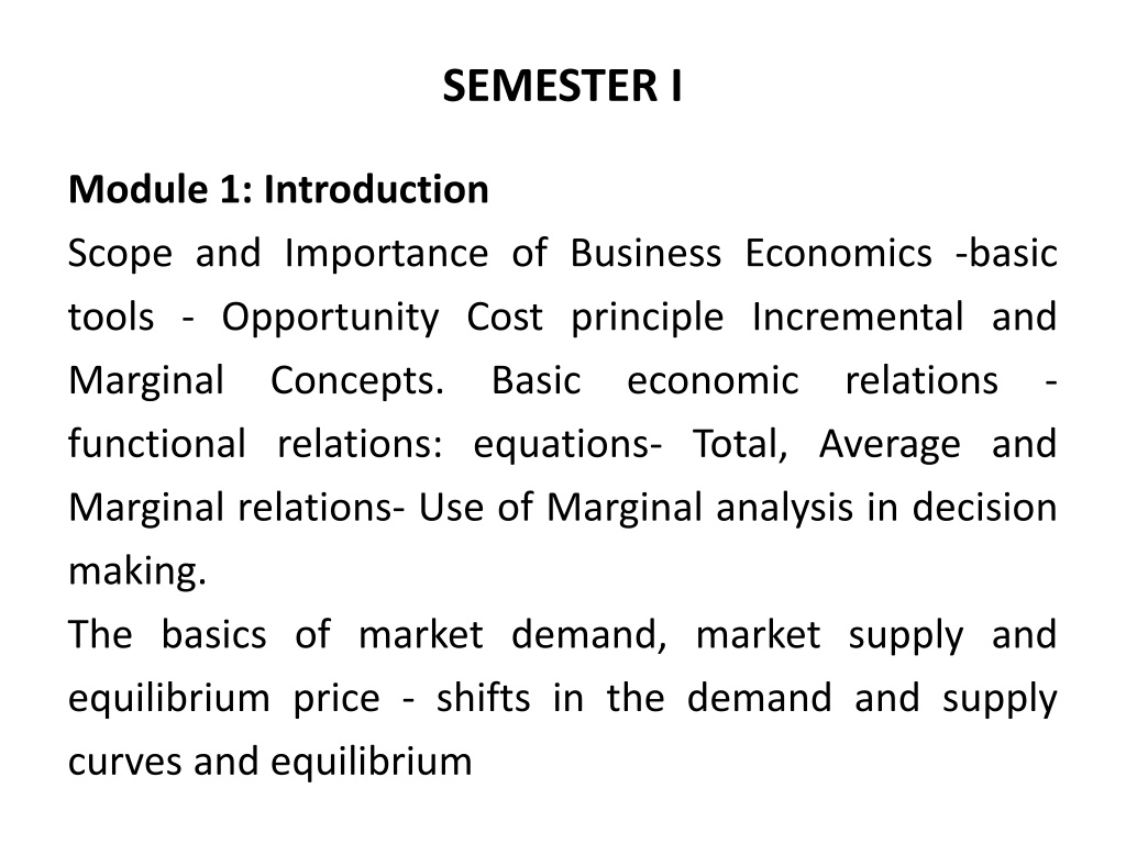
SEMESTER I Module 1: Introduction Scope and Importance of Business Economics -basic tools - Opportunity Cost principle Incremental and Marginal Concepts. Basic functional relations: equations- Total, Average and Marginal relations- Use of Marginal analysis in decision making. The basics of market demand, market supply and equilibrium price - shifts in the demand and supply curves and equilibrium economic relations -
1.1 Introduction Economics studies how societies use their scare resources to produce and distribute commodities to satisfy unlimited wants of its people. Goods and services are produced because they have utility or the capacity to satisfy human wants. Production requires resources. Resources are broadly classified into land, labour, capital and enterprise. Since resources are scare and have alternative uses, they have to be used optimally, i.e., with min. wastage. Use of scare resources involves rational choices. Economics is the science of choices. Thus the problems of scarcity and choices become the basis of economic analysis.
Microeconomics Macroeconomics 1. Macro is derived from Greek word makros meaning large . 2. It studies the functioning of an economy as a whole. 1. Micro is derived from Greek word mikros meaning small . 2. It studies the economic behaviour of individual decision making units such as consumers, resource owners, business firms, etc. 3. It examines the behaviour of the firm with regard to determination of its product price, output and employment. 4. It examines how prices of products and factors are determined and how resources are allocated among various uses. 3. It studies aggregate or collective behaviour of a society in connection with economic choices. 4. The main area of study includes national income, aggregate demand and supply, employment level, inflation, recession, international trade. 5. Business firms use macroeconomic data and analyses to formulate present and future business policies. 5. Its principles and concepts are used by firms to make decision regarding pricing, marketing, resources utilisation and profit analysis.
1.2 Scope of Business Economics Business economics is a field in economics that deals with issues such as management, expansion and strategy. The primary focus of business economics is a business enterprise or the firm. Business enterprises are units of production of goods and services whose primary objective is to produce for the market in order to earn profit. business organization,
Scope of Business Economics 1. Market Demand and Supply 2. Production Analysis 3. Cost and Profit Analysis 4. Market Structures 5. Pricing 6. Objectives of the Firm 7. Forecasts and Business Policy 8. Project Planning
Scope of Business Economics 1. Market Demand and Supply Producer or a firm produce for the market where the product price and its sales is determines with the interaction of demand and supply, which in turn determines its profit or loss (total revenue total cost). Thus, a survival of firm depends on the determination of a product price in the market.
Scope of Business Economics 2. Production Analysis: A firm always tries to make optimum use of the resources available to it in order to maximise production at minimum cost. For instance, Law of Variable Proportions and Law of Returns to Scale are used to understand production in the short run and the long run, respectively.
Scope of Business Economics 3. Cost and Profit Analysis: Business economics uses concepts of opportunity cost and implicit cost to determine economic profit and differentiate it from accounting profit. This is done to determine the actual utilisation of resources.
Scope of Business Economics 4. Market Structures: The study of market structures like perfect competition, monopoly, monopolistic competition and oligopoly help firms to take better decisions about their pricing, marketing and production strategies.
Scope of Business Economics 5. Pricing: Business economics deals with the analysis of different pricing practises and studies their application in different types of firms. For instance, which pricing practice is appropriate for a multi- product firm of a public sector enterprise?
Scope of Business Economics 6. Objectives of the Firm: Business economics studies break-even analysis and profit maximising equilibrium of a firm. It also studies objectives of the firm like, sales and growth maximisation, etc. 7. Forecasts and Business Policy: Business economics uses quantitative techniques (mathematics and statistical techniques) to study how firm forecast future trends in demand, costs, revenue and profit.
Scope of Business Economics 8. Project Planning: Project planning or capital budgeting is done by an investor to determine the criteria on which to make investment decisions. Methods like pay-back period, net present value and internal rate of return are studied under business economics.
Relationship between Economic Concepts and Business Decisions Economic Concept/Theory 1. Demand Analysis Business Economics/Decisions 1. Product, pricing, innovation, marketing 2. Input Output analysis, use of technology, productivity improvement, recycling wastes, environmental compliance 3. Price-output decisions, marketing, diversification, market expansion, mergers, takeovers 4. Investment decisions 2.Production and Cost Analysis 3.Market Structure Analysis 4.Project Appraisals 5. Firms Behaviour Analysis 5. Profit determination, sales and market share targets, stakeholders interest
1.3 Basic tools/concepts for Business Economics analysis (A) Opportunity Cost: Think about the different options you face in life, like Whether to go to college or to work? Whether to study or go out on a date? Whether to go to class or sleep in? The opportunity cost of an item is what you give up to obtain that item. The choice and sacrifice needs to be made because; resources are scarce; and resources have alternative uses. The concept of opportunity cost is used to determine factor incomes like rent, interest and wages.
1.3 Basic tools/concepts for Business Economics analysis (B) Marginalism and Incrementalism Marginalism is at the base of economic decision making. Economic choice usually involves some adjustment or change from the existing situation. Therefore, decisions regarding use of resources have to be made at the margin . This is referred to as marginalism. Marginal means addition or extra. Mathematically, marginal is denoted by a small unit change and is expressed by the symbol .
1.3 Basic tools/concepts for Business Economics analysis Incrementalism The term marginal denotes a small unit change, many a times changes take place in chunks or batches , for example, firms do not generally increase production by one more unit, but by a batch of additional units. In such situations the concept used is Incrementalism.
1.4 Relationship between Total, Average and Marginal i. Total and Marginal: Marginal measures any change in the total values. When a total value changes it is reflected in the marginal measurement. For example, changes in total utility are measured by marginal utility. Change in Total Marginal Total values are increasing Marginal values will be positive Total values are declining Total value rise at an increasing rate Marginal values will be negative Marginal values will rise Total values rise at an diminishing rate Marginal values will fall
1.4 Relationship between Total, Average and Marginal Marginal and Average: Average measures the arithmetic mean. In economics average is calculated by dividing a dependent total value by a relevant independent value. For e.g. average product (AP) is measured as total product/Units of labour used. ii. TP AP = = L The relationship between average values and marginal values can be explained as follows: (a)When marginal is greater than average, average will rise. (b)When marginal is equal to average, average will remain constant. (c)When marginal is less than average, average will fall.
1.5 Basic economic relations - functional relations: equations (a) Variable A variable is a magnitude of interest that can be defined and measures. In other words a variable is something whose magnitude can change or can take on different values. Variables frequently used in business economics are price, profit, revenue, cost, investment, etc. Since each variable can have different values, it is represented by a symbol. For instance price may be represented by P, cost by C, and so on.
1.5 Basic economic relations - functional relations: equations Variables can be endogenous and exogenous. An endogenous variable is a variable that is explained within a theory. An exogenous variable influence endogenous variables but the exogenous is itself is determined by factors outside the theory.
1.5 Basic economic relations - functional relations: equations (b) Functions A function shows the relationship between two or more variables. It indicates how the value of one variable (i.e. dependent variable) depends on the value of one or more other (i.e. independent) variables. C = f (Y) Where, C = consumption expenditure, f = functional relation and Y = disposable income (income after tax).
1.5 Basic economic relations - functional relations: equations This functional expression means that aggregate consumption depends upon the disposable income. Similarly, in business economics, functional relations between price of a commodity (P) and quantity demanded (Q) can be expressed as Q = f(P).
1.5 Basic economic relations - functional relations: equations (c) Equations An equation specifies the relationship between the dependent and independent variables. The function Q = f(P) can be expressed in the form of an equation as Q = a - bP, Where a and b are parameters and have values greater than zero.
1.5 Basic economic relations - functional relations: equations The equation shows that quantity demanded is an inverse linear function of price. The coefficient 'a' denotes quantity demanded at zero price. When the price is zero, bP will be zero, but quantity demanded will not be zero but will be equal to 'a'. In the above equation, b measures the slope of the demand curve. It is measured as Q/ P. The demand curve has a negative slope, hence the negative sign.
1.6 Market Demand and Supply 1. Equilibrium The word equilibrium is a situation where no one's likes to change. Equilibrium point is one where both supply and demand curves intersects. The price at which these two curves intersect is called the equilibrium price, and the quantity is called the equilibrium quantity.
1.6 Market Demand and Supply At the equilibrium price, the quantity of the commodity that buyers are willing and ready to buy exactly equal the quantity that sellers are willing and ready to sell. It is also known as market-clearing price because, at this price both buyers and sellers achieve maximum level of satisfaction.
1.6 Market Demand and Supply 2. Demand Demand refer to the amount of some good or service consumers are willing and able to purchase at each price. (a) Demand Schedule and Demand Curve According to the Law of Demand, "other things equal, when the price of a good rises, the quantity demanded of the good falls". In other words, there is inverse relationship between price and quantity demanded. Functionally,
1.6 Market Demand and Supply Functionally, DX = f (PX) Where, DX = Quantity demanded of commodity x PX = Price of commodity x f = functional relationship Demand in Equation form: DX = a - bPX Where, a = amount of quantity demanded, when P = 0 b = responsiveness of change in quantity demanded due to change in price or elasticity. For Example, DX = 100 - 6PX
Demand Schedule It is a table that shows the relationship between the price of a good and the quantity demanded. Quantity Demanded in Units Price/Unit (Rs.) (DX = 100 - 6PX) 0 DX = 100 - 6(0) = 10 1 DX = 100 - 6(1) = 94 2 DX = 100 - 6(2) = 88 3 DX = 100 - 6(3) = 82 4 DX = 100 - 6(4) = 76
Demand Curve D Price (Rs.) 6 5 4 3 2 1 D 0 10 203040506070 8090100 Quantity
(b) Changes in Demand 1. Movement along the demand curve: When the price of product changes, with no change in the other determinants of demand, it can be shown by movement on the same demand curve. D Price (Rs.) 6 5 B 4 3 2 1 A D 0 10 203040506070 8090100 Quantity
(b) Changes in Demand 2. Shifts in the demand curve: The demand curve will shift upward or downward when there is a change in the non-price determinants of demand. For e.g., if consumers income increase, then there will be increase in demand at the same price and the demand curve will shift upward. On the other hand, if there is fall in consumers income there will be decrease in demand at the same price and the demand curve shift downward.
(b) Changes in Demand In the diagram, DD is the initial demand curve, D1D1 shows increase in demand. At the same price P1, more is demanded (OQ1). D2D2 shows decrease in demand. At the same price P1, less is demanded (OQ2). D 1 Price (Rs.) D D 2 1 P D 1 D D 2 O Q Q Q 1 2 Quantity
1.6 Market Demand and Supply 3. Supply Supply refers to the various quantities of a commodity which producer will offer for sale at a particular time at various corresponding prices. The law of supply states that there is a direct functional relationship between the quantity supplied of a commodity and its price, other things remaining constant.
Law of Supply and Supply function As per the Law of Supply, if we assume that all factors, other than price, remain constant, we can derive a price-supply relationship in a functional form. A supply function for price can be expressed as Functionally, QSX = f (PX) Where, QSX = Quantity supplied of commodity x PX = Price of commodity x f = functional relationship
Supply Equation The above supply function in a linear form can be expressed as QSX = - c + dPX Where, c = quantity supplied when price is zero d = correlation coefficient between quantity supplied and price. Let us suppose, the supply equation is estimated as Qsx = - 40 + 30Px From the above equation, we can derive the following supply schedule:
Supply Schedule Quantity Supplied in Units Price/Unit (Rs.) (QSX = - 40 + 30PX) Qsx = - 40 + 30 (0) = - 40 Qsx = - 40 + 30 (1) = - 10 Qsx = - 40 + 30 (2) = 20 Qsx = - 40 + 30 (3) = 50 Qsx = - 40 + 30 (4) = 80 Qsx = - 40 + 30 (5) = 110 Qsx = - 40 + 30 (6) = 140 0 1 2 3 4 5 6


 Changes in Demand")
 Changes in Demand")
 Changes in Demand")