Overview of 2-Sample t-tests for Statistical Analysis

This content provides detailed information on conducting 2-sample t-tests for statistical analysis, including independent samples and test of equal variances. It covers test statistics, hypothesis testing, model assumptions, and practical examples using data from NBA and WNBA players. The material is rich in technical details and examples for applied statistical methods using R.

Download Presentation

Please find below an Image/Link to download the presentation.
The content on the website is provided AS IS for your information and personal use only. It may not be sold, licensed, or shared on other websites without obtaining consent from the author. Download presentation by click this link. If you encounter any issues during the download, it is possible that the publisher has removed the file from their server.
E N D
Presentation Transcript
R for Applied Statistical Methods Larry Winner Department of Statistics University of Florida
2-Sample t-test (Independent Samples) Case 1 Model: Note: Some introductory books use ( ) = ,sd= 2 mean we use var = N ( ) 2 1 Group 1 (Sample Size = ) : ,..., ~ , n Y Y N 1 11 1 1 n 1 ( ) 2 2 Group 2 (Sample Size = ) : ,..., ~ , n Y Y N 2 21 2 2 n 2 Data: n n n n ( ) ( ) 2 2 1 1 2 2 Y Y Y Y Y Y 1 2 1 1 2 2 j j j j = = = = 1 n 1 1 n 1 j j j j = = = = 2 1 2 2 Y s Y s 1 2 1 1 n n 1 1 2 2 = Hypothesis: : 0 : 0 H H 0 1 2 1 2 A ( ) = 2 1 2 2 Case 1: Equal Population Variances: ( ) n ( ) + n 2 1 + 2 2 1 1 n s n s Y Y 1 2 = = = + 1 2 2 p Test Statistic: where with 2 t s df n n 1 2 obs 2 ) 1 n 1 n 1 2 + 2 p s 1 2 ( ) ( = + value: 2 2 P P P t n n t 1 2 obs ( ) ( ) + 1 100% CI for : , 2 Y Y t n n 1 2 1 2 1 2 2
2-Sample t-test Case 2 and Test of Equal Variances ( ) 2 1 2 2 Case 2: Unequal Population Variances: Known as Welch's method (and Satterthwaite approx for df) 2 2 1 2 2 s n s n + Y Y 1 2 = = = 1 2 Test Statistic: with t df df ( ) ( ) obs S 2 2 2 1 2 2 s n s n 2 1 n 2 2 n s n s n + 1 1 2 1 + 1 2 1 2 ( ) ( ) = value: 2 P P P t df t S obs ( ) ( ) 1 100% CI for : , Y Y t df 1 2 1 2 S 2 Testing for Equal Variances: test: Note many packages use Levene's Test F 2 1 2 2 2 1 2 2 2 1 2 2 s = : 1 : 1 H H 0 A s = = = Test Statistic: with 1, 1 F df n df n 1 1 2 2 obs 1 ( ) ( ) ( ) = value: 2min 1, 1 , 1, 1 P P P F n n F P F n n 1 2 2 1 obs F obs 2 1 2 2 2 1 2 2 s s s s 2 1 2 2 1 ( ) = 1 100% CI for : , whe re: 1 ; 1, 1 F n n 1 2 2 ; 1, 1 1 ; 1, 1 ; 1, 1 F n n F n n F n n 1 2 1 2 2 1 2 2 2
Example NBA and WNBA Players BMI Groups: Male: NBA(i=1) and Female: WNBA(i=2) Samples: Random Samples of n1= n2= 20 from 2013 seasons (2013/2014 for NBA) lbs kg = = 703 BMI = = 2 1 Males: =20 24.9466 = 3.0919 = n Y s 1 1 2 2 inches metres 2 2 Females: =20 23.3510 4.2694 n Y s 2 2 Player Giannis Antetokounmpo Joel Anthony Alex Len Erik Murphy Ersan Ilyasova Kevin Garnett Chauncey Billups Juwan Howard Vladimir Radmanovic Tiago Splitter Jarvis Varnado Alexey Shved Jermaine O`Neal Michael Kidd-Gilchrist Metta World Peace Tim Hardaway Jr. Greivis Vasquez Daniel Gibson Terrence Ross Chris Kaman id Gender Height Weight BMI Player id Gender Height Weight BMI 1 2 3 4 5 6 7 8 9 1 1 1 1 1 1 1 1 1 1 1 1 1 1 1 1 1 1 1 1 81 81 85 82 82 83 75 81 82 83 81 78 83 79 79 78 78 74 79 84 205 245 255 230 235 253 202 250 235 240 230 190 255 232 260 205 211 200 197 265 21.97 Tamika Catchings 26.25 Courtney Clements 24.81 Allie Quigley 24.05 Quanitra Hollingsworth 24.57 Katie Smith 25.82 Tayler Hill 25.25 Allison Hightower 26.79 Kara Braxton 24.57 Eshaya Murphy 24.49 Michelle Campbell 24.64 Briann January 21.95 Jasmine James 26.02 Kelsey Bone 26.13 Jia Perkins 29.29 Ebony Hoffman 23.69 Shavonte Zellous 24.38 Matee Ajavon 25.68 Karima Christmas 22.19 Erika de Souza 26.40 Jayne Appel 21 22 23 24 25 26 27 28 29 30 31 32 33 34 35 36 37 38 39 40 2 2 2 2 2 2 2 2 2 2 2 2 2 2 2 2 2 2 2 2 73 72 70 77 71 70 70 78 71 74 68 69 76 68 74 70 68 72 77 76 167 22.03059 155 21.01948 140 20.08571 203 24.06966 175 24.40488 145 20.80306 139 19.94224 225 25.99852 164 22.87086 183 23.49324 144 21.89273 175 25.84016 200 24.34211 155 23.5651 215 27.60135 155 22.23776 160 24.32526 180 24.40972 190 22.52825 210 25.55921 Note: Actual data file has males stacked over Females. See next slide. 10 11 12 13 14 15 16 17 18 19 20
Data File (.csv) Player Giannis Antetokounmpo Joel Anthony Alex Len Erik Murphy Ersan Ilyasova Kevin Garnett Chauncey Billups Juwan Howard Vladimir Radmanovic Tiago Splitter Jarvis Varnado Alexey Shved Jermaine O`Neal Michael Kidd-Gilchrist Metta World Peace Tim Hardaway Jr. Greivis Vasquez Daniel Gibson Terrence Ross Chris Kaman Tamika Catchings Courtney Clements Allie Quigley Quanitra Hollingsworth Katie Smith Tayler Hill Allison Hightower Kara Braxton Eshaya Murphy Michelle Campbell Briann January Jasmine James Kelsey Bone Jia Perkins Ebony Hoffman Shavonte Zellous Matee Ajavon Karima Christmas Erika de Souza Jayne Appel Gender Height Weight BMI 1 1 1 1 1 1 1 1 1 1 1 1 1 1 1 1 1 1 1 1 2 2 2 2 2 2 2 2 2 2 2 2 2 2 2 2 2 2 2 2 81 81 85 82 82 83 75 81 82 83 81 78 83 79 79 78 78 74 79 84 73 72 70 77 71 70 70 78 71 74 68 69 76 68 74 70 68 72 77 76 205 245 255 230 235 253 202 250 235 240 230 190 255 232 260 205 211 200 197 265 167 155 140 203 175 145 139 225 164 183 144 175 200 155 215 155 160 180 190 210 21.9654 26.25133 24.81176 24.0467 24.56945 25.81783 25.24551 26.78708 24.56945 24.49122 24.64411 21.95431 26.02192 26.13299 29.28697 23.68754 24.38083 25.67568 22.19051 26.40235 22.03059 21.01948 20.08571 24.06966 24.40488 20.80306 19.94224 25.99852 22.87086 23.49324 21.89273 25.84016 24.34211 23.5651 27.60135 22.23776 24.32526 24.40972 22.52825 25.55921
t-test for NBA vs WNBA BMI Equal Variances = : 0 : 0 H H 0 1 2 1 2 A ( ) Y Y H 1 2 ( ) 0 = + : ~ 2 TS t t n n 1 2 obs 1 n 1 n + 2 p s 1 2 Data (From EXCELSpreadsheet): = = = = = = = 2 1 2 2 20 20 1 3.0919 24.9466 + + 23.3510 3.0919 4.2694 n n Y Y s s 1 2 1 2 ( ) ( ) 20 1 4.2694 = 2 p 3.6806 s 20 20 2 ( ) 24.9466 23.3510 0 = = 2.6301 t obs 1 20 1 20 + 3.6806 ( ) ( ) P value = = :2 38 2.6301 2(.0061) .0122 P t
t-test for NBA vs WNBA BMI Unequal Variances = : 0 : 0 H H 0 1 2 1 2 A 2 2 1 2 2 s n s n + Y Y 1 2 = = 1 2 Test Statistic: with t df ( ) ( ) obs 2 2 2 1 2 2 s n s n 2 1 n 2 2 n s n s n + 1 1 2 1 + 1 2 1 2 24.9466 3.0919 20 23.3510 4.2694 20 Y Y 1 2 = = = 2.6301 t obs 2 1 2 2 s n s n + + 1 2 2 3.0919 20 4. 2694 20 4.2694 20 20 1 + 0.135472 0.003656 = = = 37.05 df ( ) ( ) 2 2 3.0919 20 20 1 + ( ) ( ) = = :2 37 2.6301 2(.0062) .0124 P value P t Note: the test statistics are the same (n1 = n2) and the degrees of freedom very close (s1 s2)
Test for Equal Variances for WNBA vs NBA BMI = = = = 2 1 2 2 Data: 20 3.0919 20 4.2694 n s n s 1 2 = = = = = 20 1 19 : = Critical F-values 0.05 0.025 1 0.975, df df 1 2 2 2 1 ( ) ( ) = = = 0.025;19,19 2.5265 0.975;19,19 0.3958 F F 2.5265 2 1 2 2 2 1 2 2 2 1 2 2 s = : 1 : 1 H H 0 A 3.0919 4.2694 s = = = Test Statistic: 0.7242 F obs 1 ( ) ( ) ( ) = value: 2min 19,19 0.7242 , 19,19 P P P F P F 0.7242 ( ) = = 2min 0.7557, 0.2443 2(0.2443) 0.4886 2 1 2 2 0.7242 2.5265 0.7242 0.3958 ( ) 1 100% CI for : , 0.2866, 1.8297
Small Sample Test to Compare Two Medians Non-Normal Populations Two Independent Samples (Parallel Groups) Procedure (Wilcoxon Rank-Sum Test): Null hypothesis: Population Medians are equal H0: M1 = M2 Rank measurements across samples from smallest (1) to largest (n1+n2). Ties take average ranks. Obtain the rank sum for group with smallest sample size (T ) 1-sided tests: Conclude HA: M1 > M2if T > TU Conclude: HA: M1 < M2if T < TL 2-sided tests: Conclude HA: M1 M2if T > TU or T < TL Values of TL and TU are given in tables for various sample sizes and significance levels (Some tables use T=Rank sum for larger Group). This test gives equivalent conclusions as Mann-Whitney U-test
Rank-Sum Test: Normal Approximation Under the null hypothesis of no difference in the two groups (let T be rank sum for group 1): + + ( 1) ( 12 1) n N 1 2 n n N = = = + N n n 1 1 2 T T 2 A z-statistic can be computed and P-value (approximate) can be obtained from Z-distribution + + ( 1)/ 2 1)/12 T T n N = = z 1 ( T obs 1 2 n n N T Note: When there are many ties in ranks, a more complex formula for T is often used, with little effect unless there are many ties.
WNBA/NBA BMI Data Wilcoxon Rank-Sum Test Player Giannis Antetokounmpo Joel Anthony Alex Len Erik Murphy Ersan Ilyasova Kevin Garnett Chauncey Billups Juwan Howard Vladimir Radmanovic Tiago Splitter Jarvis Varnado Alexey Shved Jermaine O`Neal Michael Kidd-Gilchrist Metta World Peace Tim Hardaway Jr. Greivis Vasquez Daniel Gibson Terrence Ross Chris Kaman Tamika Catchings Courtney Clements Allie Quigley Quanitra Hollingsworth Katie Smith Tayler Hill Allison Hightower Kara Braxton Eshaya Murphy Michelle Campbell Briann January Jasmine James Kelsey Bone Jia Perkins Ebony Hoffman Shavonte Zellous Matee Ajavon Karima Christmas Erika de Souza Jayne Appel id Gender Height Weight BMI Rank 1 2 3 4 5 6 7 8 9 1 1 1 1 1 1 1 1 1 1 1 1 1 1 1 1 1 1 1 1 2 2 2 2 2 2 2 2 2 2 2 2 2 2 2 2 2 2 2 2 81 81 85 82 82 83 75 81 82 83 81 78 83 79 79 78 78 74 79 84 73 72 70 77 71 70 70 78 71 74 68 69 76 68 74 70 68 72 77 76 205 245 26.25133 255 24.81176 230 24.0467 235 24.56945 253 25.81783 202 25.24551 250 26.78708 235 24.56945 240 24.49122 230 24.64411 190 21.95431 255 26.02192 232 26.13299 260 29.28697 205 23.68754 211 24.38083 200 25.67568 197 22.19051 265 26.40235 167 22.03059 155 21.01948 140 20.08571 203 24.06966 175 24.40488 145 20.80306 139 19.94224 225 25.99852 164 22.87086 183 23.49324 144 21.89273 175 25.84016 200 24.34211 155 23.5651 215 27.60135 155 22.23776 160 24.32526 180 24.40972 190 22.52825 210 25.55921 21.9654 7 36 27 16 7 36 ... 9 37 = + + + + = = = = 507 20 40 T n n N 1 2 24.5 31 28 38 24.5 23 26 + 20(41 1) 2 T = (20)(20)(41) 12 97 36.9685 = = = = = 410 1366.667 T T 507 410 1366.667 2.6239 P Z 10 11 12 13 14 15 16 17 18 19 20 21 22 23 24 25 26 27 28 29 30 31 32 33 34 35 36 37 38 39 40 = = = = 2.6239 z T obs 6 34 35 40 15 20 30 9 37 8 4 2 17 21 3 1 33 12 13 5 32 19 14 39 10 18 22 11 29 T ( ) value 2 .0087 P R uses a different algorithm for a slightly different P-value. 1 ( ) + n n = 1 1 2 Note: The statistic R computes is W T This is difference between and the minimum it could be. 1 20(21) 507 2 T ( ) + n n = = = 507 210 = 1 1 2 297 W T
R Program and Output bmi1 <- read.csv("http://www.stat.ufl.edu/~winner/data/wnba_nba_bmi.csv",header=T) attach(bmi1); names(bmi1) tapply(BMI,Gender,mean) # Obtain mean BMI by Gender tapply(BMI,Gender,var) # Obtain variance of BMI by Gender tapply(BMI,Gender,length) # Obtain sample size of BMI by Gender t.test(BMI~Gender,var.equal=T) # t-test with Equal Variances t.test(BMI~Gender) # t-test with Unequal Variances var.test(BMI~Gender) # F-test for Equal Variances wilcox.test(BMI~Gender) # Wilcoxon Rank-Sum Test ################################# > tapply(BMI,Gender,mean) # Obtain mean BMI by Gender 1 2 24.94665 23.35099 > tapply(BMI,Gender,var) # Obtain variance of BMI by Gender 1 2 3.091871 4.269420 > tapply(BMI,Gender,length) # Obtain sample size of BMI by Gender 1 2 20 20
R Output (Continued) > t.test(BMI~Gender,var.equal=T) # t-test with Equal Variances Two Sample t-test data: BMI by Gender t = 2.6301, df = 38, p-value = 0.01226 alternative hypothesis: true difference in means is not equal to 0 95 percent confidence interval: 0.3674868 2.8238189 sample estimates: mean in group 1 mean in group 2 24.94665 23.35099 > t.test(BMI~Gender) # t-test with Unequal Variances Welch Two Sample t-test data: BMI by Gender t = 2.6301, df = 37.052, p-value = 0.01236 alternative hypothesis: true difference in means is not equal to 0 95 percent confidence interval: 0.3664539 2.8248518 sample estimates: mean in group 1 mean in group 2 24.94665 23.35099
R Output (Continued) > var.test(BMI~Gender) # F-test for Equal Variances F test to compare two variances data: BMI by Gender F = 0.7242, num df = 19, denom df = 19, p-value = 0.4885 alternative hypothesis: true ratio of variances is not equal to 1 95 percent confidence interval: 0.2866432 1.8296302 sample estimates: ratio of variances 0.7241899 > wilcox.test(BMI~Gender) Wilcoxon rank sum test with continuity correction data: BMI by Gender W = 297, p-value = 0.009042 alternative hypothesis: true location shift is not equal to 0 Warning message: In wilcox.test.default(x = c(21.96540162, 26.25133364, 24.81176471, : cannot compute exact p-value with ties
Paired t-test Setting: n matched pairs, each under 1 of 2 competing conditions Note: In many experiments, it is the same Subject under each condition = = Data: 1,..., Difference between measurement unde n ( j d d r Conditions 1 and 2 d Y Y j 1 2 j j j ) n n 2 d j = = 1 n 1 j j = = 2 d d s 1 n = = = : 0 : 0 H H 0 1 d s 2 1 2 d A d = = : with 1 TS t df n obs 2 d n P ( ) ( ) = value: 2 1 P P t n t obs 2 d s n ( ) = 1 100% CI for : ; 1 d t n 1 2 d 2
Example: English Premier League Football - 2012 Interested in Determining if there is a home field effect League has 20 teams, all play all 19 opponents Home and Away (190 pairs of teams, each playing once on each team s home field). No overtime. We are treating each pair of teams as a unit Y1 is the Total Score for the Home Teams, Y2 is for Away Note: d represents combined Home Goals Combined Away Goals for the Pair of teams ( units ) No home effect should mean d = 0 Programming Note: In Independent Sample t-test, we had a Variable for Treatment/Group and another variable for Response (Y). Here we have Y1 and Y2 as separate variables, with each row as a unit
Portion of Data File (.csv). Note n =190 Team1 Arsenal Arsenal Arsenal Arsenal Arsenal Arsenal Arsenal Arsenal Arsenal Arsenal Arsenal Arsenal Arsenal Arsenal Arsenal Arsenal Arsenal Arsenal Arsenal Aston Villa Team2 Aston Villa Chelsea Everton Fulham Liverpool Manchester City Manchester United Newcastle United Norwich City Queens Park Rangers Reading Southampton Stoke City Sunderland Swansea City Tottenham Hotspur West Bromwich Albion West Ham United Wigan Athletic Chelsea Home Away 2 3 1 3 2 1 3 7 4 1 6 7 1 0 0 7 3 6 4 9 1 3 1 4 4 3 2 4 1 1 6 2 0 1 4 3 2 4 2 2
Paired t-test for EPL 2012 Home vs Away Goals = = = : 0 : 0 H H 0 1 d s 2 1 2 d A d = = : with 1 TS t df n obs 2 d n = = = 2 d Data (From EXCEL Spreadsheet): 0.6368 4.3912 190 value:2 189 P P t 190 0.6368 4.3912 n d s = = 4.1888 t obs ( ) ( ) = = 4.1888 2(.00002) .00004 4 .3912 190 = 0.6368 0.2999 95:% CI for : 0.6368 1.9726 d ( ) 0.3369, 0.9367
R Program / Output epl.2012 <- read.csv("http://www.stat.ufl.edu/~winner/data/epl_2012_home.csv", header=T) attach(epl.2012); names(epl.2012) t.test(Home,Away,paired=T) wilcox.test(Home,Away,paired=T) ####################### > t.test(Home,Away,paired=T) Paired t-test data: Home and Away t = 4.1891, df = 189, p-value = 4.294e-05 alternative hypothesis: true difference in means is not equal to 0 95 percent confidence interval: 0.3369575 0.9367267 sample estimates: mean of the differences 0.6368421
Small-Sample Test For Nonnormal Data Paired Samples (Crossover Design) Procedure (Wilcoxon Signed-Rank Test) Compute Differences di (as in the paired t-test) and obtain their absolute values (ignoring 0s). n= number of non-zero differences Rank the observations by |di| (smallest=1), averaging ranks for ties Compute T+ and T- , the rank sums for the positive and negative differences, respectively 1-sided tests:Conclude HA: M1 > M2if T=T- T0 2-sided tests:Conclude HA: M1 M2if T=min(T+ , T-) T0 Values of T0 are given in various tables for various sample sizes and significance levels. Some tables give the upper tail cut-off T0 values P-values are printed by statistical software packages.
Signed-Rank Test: Normal Approximation Under the null hypothesis of no difference in the 2 groups: Let T = T+ + + + ( 1) ( 1)(2 24 1) n n n n n = = T T 4 Z-Statistic computed and approximate P-value can be obtained from: + + ( 1)/ 4 1)/ 24 + T T n n = = z T obs ( 1)(2 n n n T When there are ties (many common ds) as in soccer data, T is reduced and is of form: g ( ) 1 24 1 2 ( )( ) ( )( ) = + + + 1 2 1 1 1 n n n t t t T j j j = 1 t where: # of distinct levels of and is the # of ties at level d g t j j
EPL Home Field Advantage Zero differences have been removed Diff (d) Count (t) T+ -6 -4 -3 -2 -1 1 2 3 4 5 7 1 3 7 0 0 0 0 0 T+ E(T) sigma^2_T sigma_T Z p-value 7896.5 5738 283006 531.98 4.0575 0.0000496 17 27 30 33 16 10 6 1 151 The Differences and their Counts are at top left 29 82.5 119 137 146.5 151 Absolute differences and their counts and average ranks are at bottom sum T+ is the sum of the products of the counts and the T+ columns (e.g. There are 30 cases with d=+1, each getting rank=29) |Diff| Count(t) LowRank 57 50 23 13 6 1 1 HighRank MeanRank t(t-1)*(t+1) 29 82.5 119 137 146.5 150 151 1 2 3 4 5 6 7 1 57 107 130 143 149 150 151 185136 124950 12144 2184 210 58 108 131 144 150 151 0 0 The Z is large and P-value is small 324624 R Labels T+ as V
R Output > wilcox.test(Home,Away,paired=T) Wilcoxon signed rank test with continuity correction data: Home and Away V = 7896.5, p-value = 4.981e-05 alternative hypothesis: true location shift is not equal to 0
Test for Association for Categorical Variables Counts Col 1 Col 2 Col c Total Row 1 n11 n21 n12 n22 n1c n2c n1 n2 Row 2 Row r nr1 n 1 nr2 n 2 nrc n c nr n Total n n ^ n i n j = = = Expected Cell Counts: 1,..., ; 1,..., i r j c ij 2 ^ n n ij ij r c ( )( ) = = 2 P Pearson Chi-Square Statistic: 1 1 X df r c ^ n = = 1 1 i j ij n r c ( )( ) ij = = 2 LR Likelihood-Ratio Chi-Square Statistic: 2 ln 1 1 X n df r c ij ^ n = = 1 1 i j ij Reject the null hypothesis of no association between the row and column variables if: ( ) ( ) ( )( ) ( )( ) = 2 2 2 2 ; 1 1 value: 1 1 X r c P P P r c X
Example: Crop Circles by Country and Field Type n n ^ n i n j = = = Expected Cell Counts: 1,...,9; 1,2 i j ij Observed Country England Germany Italy USA Canada Holland Switzerland Belgium Czech Republic Total Percent 431(297) 863 n n ^ n other wheat Total = = = = For England/other (i=1 , j=1): 148.33 with 108 n 1 n 1 11 11 108 47 56 27 32 10 323 90 46 17 11 24 23 18 14 566 431 137 102 44 43 34 29 22 21 863 100 2 ^ n n ij ij r c = 2 P Pearson Chi-Square Statistic: X ^ n = = 1 1 i j ij 2 = ^ n n ( ) 2 11 108 148.33 148.33 11 6 4 7 = Contribution from cell with England/other: 10.97 ^ n 11 n r c ij = 2 LR Likelihood-Ratio Chi-Square Statistic: 2 ln X n 297 ij ^ n = = 1 1 i j 34.41483 65.58517 ij = 108 148.33 n = Contribution from cell with England/o ther: 2 ln 2(108)ln 68.54 n 11 11 ^ n Both tests are highly significant. 11 Pearson Chi-square Country England Germany Italy USA Canada Holland Switzerland Belgium Czech Republic Total Expected Country England Germany Italy USA Canada Holland Switzerland Belgium Czech Republic Total Likelihood-Ratio Chi-Square Country England Germany Italy USA Canada Holland Switzerland Belgium Czech Republic Total wheat0 10.9645 5.753457 16.71796 0.000467 0.000245 0.000711 12.43989 6.527648 18.96754 9.285088 4.872211 19.99515 10.49216 30.48731 0.24729 0.129762 0.377051 1.587407 0.832968 2.420375 1.684517 0.883925 2.568442 0.007137 0.003745 0.010882 56.21145 29.49612 85.70757 wheat1 Total wheat0 148.3279 282.6721 47.14832 89.85168 35.10313 66.89687 15.14253 28.85747 14.79838 28.20162 11.70104 22.29896 9.980301 7.571263 14.42874 7.227115 13.77289 297 wheat1 Total wheat0 -68.5356 86.15369 17.61812 -0.29617 0.296884 0.000712 52.31088 -34.455 17.85589 31.22981 -17.9913 13.23852 49.35797 -20.7127 28.64532 -3.14186 3.528668 0.386811 -6.10625 8.740874 2.634628 -5.10452 7.961397 2.856873 -0.44702 0.457954 0.010938 49.26727 33.98053 wheat1 Total 431 137 102 44 43 34 29 22 21 863 14.1573 19.0197 83.2478 85.70757 X^2(obs) 15.50731 X^2(.05,8) 566
R Program Uses the vcd Package cc <- read.csv("http://www.stat.ufl.edu/~winner/data/crop_circle",header=T) attach(cc); names(cc) (wheat.country <- table(Country,wheat)) chisq.test(wheat.country) install.packages("vcd") library(vcd) assocstats(wheat.country) barplot(wheat.country, col=c("blue","green","pink","purple","red", "yellow","orange","cornflowerblue","beige"), main="Wheat by Country",xlab="Wheat",ylab="Count") labs <- rownames(wheat.country) legend(locator(1),labs,fill=c("blue","green","pink","purple","red", "yellow","orange","cornflowerblue","beige")) barplot(wheat.country,beside=T, col=c("blue","green","pink","purple","red", "yellow","orange","cornflowerblue","beige"), main="Wheat by Country",xlab="Wheat",ylab="Count") labs <- rownames(wheat.country) legend(locator(1),labs,fill=c("blue","green","pink","purple","red", "yellow","orange","cornflowerblue","beige"))
R Output > (wheat.country <- table(Country,wheat)) wheat Country 0 1 Belgium 4 18 Canada 32 11 Czech 7 14 England 108 323 Germany 47 90 Holland 10 24 Italy 56 46 Swiss 6 23 USA 27 17 ################################################## > assocstats(wheat.country) X^2 df P(> X^2) Likelihood Ratio 83.248 8 1.0880e-14 Pearson 85.708 8 3.4417e-15 Phi-Coefficient : 0.315 Contingency Coeff.: 0.301 Cramer's V : 0.315

 – Case 1")


")


")
")


. Note n =190")