Understanding Sample Size, Power, and Hypothesis Testing in Statistics

Sample size determination based on estimation precision and confidence interval width is crucial in statistical analysis. By calculating the necessary sample size, researchers can ensure sufficient standard errors and confidence intervals. Additionally, the relationship between power and sample size in hypothesis testing plays a vital role in making accurate decisions in research. Understanding determinants of power, alpha versus power, and the implications of statistical versus medical testing further enriches one's grasp of statistical concepts.

Uploaded on Sep 16, 2024 | 0 Views
Download Presentation

Please find below an Image/Link to download the presentation.
The content on the website is provided AS IS for your information and personal use only. It may not be sold, licensed, or shared on other websites without obtaining consent from the author. Download presentation by click this link. If you encounter any issues during the download, it is possible that the publisher has removed the file from their server.
E N D
Presentation Transcript
Section 5 Sample Size and Power Multiple hypothesis testing
Sample size (n) based on estimation precision-CI width Can plan sample size so that standard errors (SEs) and the corresponding confidence intervals are sufficiently small. (How small? How small do you need it to be?)
Sample size for precision/CIs = proportion with TB in the population (prevalence) p = proportion with TB in a sample of size n, SE(p) = [ (1- )/n] 95% confidence interval for : p 1.96(SE) Precision: want to estimate true prevalence ( ) within 6% Solve for n: 1.96(SE) = 1.96 [ (1- )/n] = 0.06 n = 1.962 (1- )/(0.06)2= 3.84 (1- )/0.0036 Can estimate using the observed p or use maximum at =0.5 If =0.15, n = 3.84 (0.15)(0.85)/0.0036 = 136 At =0.50, n = 3.84 (0.50)(0.50)/0.0036 = 267 (worst case) Rule of thumb: For 95% CI for , conservative n for precision w is n = 1/w2
Power and Sample size based on hypothesis testing
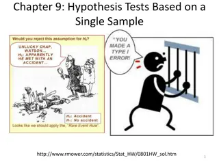
Hypothesis test decision table No difference in population (Null is true) Actual difference (Null is false) Test: Do not reject null p value > 1- (correct) (Type II error) Test: Reject null hypothesis p value < 1- = power (correct) (Type I error)
Statistical vs medical testing Medical testing: Person really has disease or does not-truth Null true~no disease, Null false~disease Person tests positive or negative ( p value < or p value ) 1- is like specificity is like false positive 1- is like sensitivity=power is like false negative
Determinants of power Power (1- ) depends on = delta = true difference = sigma = true SD or true variation = alpha = significance criterion n = sample size (Or, n depends on , , , 1- )
Alpha versus Power The top distribution shows the sampling distribution of a test statistic under the assumption that delta ( ) is zero. The null hypothesis is true. -3.0 -2.0 -1.0 0.0 1.0 2.0 3.0 The bottom distribution shows the true sampling distribution (unknown at the time of testing), with a true population delta=2.5. The null hypothesis is false. 1 - 1 - -1.0 0.0 1.0 2.0 3.0 4.0 5.0 6.0
Power calculation Zpower = Zobs Z1- /2 = ( /SE) Z1- /2 Treatment n Mean HBA1c chg -1.24 -0.90 0.34= SD SE Liraglutide Sitaglipin Difference 5 4 0.99 0.98 0.44 0.49 [0.442 + 0.492] = 0.66 Zobs=0.34/0.66 = 0.516 (<1.96, so not statistically significant, p=0.622) Zpower = Zobs - Z = 0.516 1.96 = -1.44 From the Gaussian table or EXCEL, Zpower=-1.44 yields power about 7%.
Interpretation of power If test is statistically significant (p < ), we have a positive or significant outcome & accept the false positive probability of . If test is not statistically significant (p > ) either there is no relationship ( negative outcome) or sample size is inadequate (inconclusive outcome). If power is low for a given , results are inconclusive, not negative. If power is high, results are affirmatively negative. (But better to quote Confidence interval after the study is published)
Sample size to test difference between 2 means (this is NOT a universal formula) Two independent groups, each with sample size n = 2(Zpower+ Z1- /2)2 ( / )2 Z0.975 = 1.96 and Zpower = 0.842 (for power of 80%), so n = 2(0.842 + 1.96)2 ( / )2 = 15.7 ( / )2 or n per group approximately (range/ )2 (since 15.7 16, 16( / )2 = (4 / )2and the range 4 )
Power for increasing delta =2.5 = 0 = 3.5 -3 -2 -1 0 1 2 3 4 5 6 7 Areas under the curves and right of the vertical line are for the black curve and power for the other curves. The power is larger for the red curve than for the blue.
Power Summary Power increases as: True difference ( ) increases Sample size (n) increases increases (less strict significance criterion) Patient heterogeneity ( ) decreases Generally, we set = 0.05 & power = 1 = 0.80. To determine n, we need to estimate and . Often we use values of / for the calculation For time to event outcomes (survival), n also depends on follow up time since n is the number of events. The sample size for comparing two survival curves is often computed based on comparing the corresponding two hazards.
Sample Size (n) Checklist Sample size (n) depends on: Effect size ( ) = smallest clinically important difference - n increases as decreases Variability ( ) = patient heterogeneity - n increases as variability increases Power (1- ) = probability of significantly detecting the effect (prob p value < ), often set at 80% or higher - n increases as required power increases level = probability of rejecting when is equal to its null value (often =0), (two sided often set to 0.05) - n increases with smaller - smaller is more stringent Must also consider the percent who will agree to participate and the accrual rate if all patients are not recruited at the same time. *** for time to event (survival) outcomes *** Follow up time = time each patient is followed - n decreases if patients are followed longer. In survival n is the number who have the outcome/event. There are more events if follow up time is increased. For time to event outcomes, must also consider the patient dropout / loss rate
Sample size per group for / -unpaired 2 mean comparison, mean difference= , SD= , two-sided =0.05 / 0.10 70% power 1,234 80% power 1,570 90% power 2,102 0.15 549 698 934 0.20 0.25 0.50 0.75 1.00 1.25 1.50 309 198 49 22 12 8 5 392 251 63 28 16 10 7 525 336 84 37 21 13 9
Sample size per group for comparing two proportions, 80% power, alpha=0.05 Difference between P1 and P2 |P1- P2|= 0.05 0.10 434 140 Smaller of P1 & P2 0.15 71 0.20 45 0.05 0.10 685 199 99 62 0.15 904 250 120 72
Power/sample size calculators Gpower University of Dusseldorf (free download) https://www.psychologie.hhu.de/arbeitsgruppen/allgemeine- psychologie-und-arbeitspsychologie/gpower.html Columbia University http://www.biomath.info/power/ttest.htm Harvard University (Hedwig) http://hedwig.mgh.harvard.edu/sample_size/
Hypothesis testing limitations
Pseudo replication Most variation is between persons, not within person. Two blood samples on n=10 is not a sample size of 20. Observed value = true population mean + between person variation ( p) + within person variation ( e) Example: To estimate the mean 1. Compute a mean for each person using her m observations per person. 2. Compute the group mean from the n person means. SEM = [ p2/n + e2/nm], usually e < p
Statistical vs Medical significance ( A difference, in order to be a difference, must make a difference Gertrude Stein?). Average drop in weight (kg) after 3 months Diet Mean Drop p 95% CI I 0.50 <0.001 (0.45,0.55) II 10.0 0.16 (-5.0, 25.0)
p value limitations (ASA) 1. p values do not measure the probability that the studied hypothesis is true, or the probability that the data were produced by random chance alone ignoring the model. 2. Conclusions should not be based only on whether a p- value passes a specific threshold. 3. Proper inference requires full reporting & transparency. 4. A p-value does not measure the size of an effect or the importance of a result. 5. A p-value alone does not provide a good measure of evidence regarding a model or hypothesis. 21
R A Fisher on p values Statistical Methods and Scientific Inference, Hafner, New York, ed. 1, 1956 The concept that the scientific worker can regard himself as an inert item in a vast co-operative concern working according to accepted rules, is encouraged by directing attention away from his duty to form correct scientific conclusions, and by stressing his supposed duty to mechanically make a succession of automatic decisions (ie p< 0.05). ...The idea that this responsibility can be delegated to a giant computer programmed with Decision Functions belongs to a phantasy of circles, rather remote from scientific research . [pp. 104 105]
Multiple Hypothesis testing Multiple efficacy endpoints /outcomes Multiple safety endpoints/outcomes Multiple treatment arms and/or doses Multiple interim analyses Multiple patient subgroups Multiple analyses
Exploratory vs confirmatory protein example 750 proteins are compared between two groups 12 are significant at p < 0.05 Protein name Atril fib 33.3% 38.9% 22.2% 16.7% 11.1% 11.1% 11.1% 16.7% 5.6% 27.8% 27.8% 77.8% 38.9% 94.4% 50.0% 1.0% 1.0% 1.0% 100.0% p value 0.0000 0.0000 0.0000 0.0000 0.0000 0.0000 0.0000 0.0000 0.0006 0.0013 0.0013 0.0037 0.1142 0.4402 1.0000 1.0000 1.0000 1.0000 1.0000 Atherosclerosis RAS guanyl-releasing protein 2 Glutathione S-transferase P Selenium-binding protein 1 Nucleosome assembly protein 1-like 4 Integrin beta;Integrin beta-2 Spectrin alpha chain, non-erythrocytic 1 Pituitary tumor-transforming gene 1 protein-interacting WW domain-binding protein 2 Syntaxin-4 CD9 antigen ATP synthase-coupling factor 6, mitochondrial Flotillin-1 Aconitate hydratase, mitochondrial Fructose-bisphosphate aldolase C Alpha-adducin 40S ribosomal protein SA Abl interactor 1 Bone marrow proteoglycan;Eosinophil granule major basic Tubulin alpha-4A chain (750 proteins total) 0.0% 100.0% 0.0% 0.0% 50.0% 0.0% 0.0% 50.0% 0.0% 50.0% 50.0% 100.0% 50.0% 100.0% 50.0% 1.0% 1.0% 1.0% 100.0%
Prevagen & multiple testing (Washington Post 11 Sept 2021) Does the supplement Prevagen improve memory? A court case is asking that question Quincy Bioscience describes the study as a randomized, double-blinded, placebo-controlled trial. But, according to the FTC and the New York attorney general, the trial involved 218 subjects taking either 10 milligrams of Prevagen or a placebo and failed to show a statistically significant improvement in the treatment group over the placebo group on any of the nine computerized cognitive tasks.
The complaint alleges that after the Madison Memory Study failed to find a treatment effect for the sample as a whole, Quincy s researchers broke down the data in more than 30 different ways. Given the sheer number of comparisons run and the fact that they were post hoc, the few positive findings on isolated tasks for small subgroups of the study population do not provide reliable evidence of a treatment effect, the lawsuit said. Post hoc studies are not uncommon but are generally not regarded as proof until confirmed, scientific experts say. According to the Center for Science in the Public Interest, which filed an amicus brief in support of the agencies charges, the subsequent analyses produced three results that were statistically significant (and more than 27 results that weren t).
Exploratory vs confirmatory Who killed Tweety Bird?
Motivation (class discussion) Tweety Bird is murdered by a cat who left a DNA sample. The particular DNA profile found in the sample is known to occur in one of every one million cats. There is also about a 0.01% false positive rate for this test. Is the level of evidence (guilt) equal in these two scenarios? 1. Sylvester was under suspicion for killing a bird before so Sylvester only is tested and is a match. 2. A DNA database on 100,000 cats (but not all cats), including Sylvester, is searched and Sylvester is a match, although not necessarily the only match. No prior belief that Sylvester is guilty.
Motivation (class discussion) The disease score ranges from 2 (good) to 12 (worst). Scenario A: Due to prior suspicion (prior information), only patients 19 and 47 are measured and both have scores of 12. We report that they are significantly ill. Scenario B: The score is measured on 72 patients. Only patients 19 and 47 have scores of 12. We report that they are significantly ill.
Is the amount of evidence or belief that patients 19 and 47 really are very ill (have true score of 12) the same in both scenarios? The data for patients 19 and 47 are the same in both scenarios. Most would agree that, if both patients were retested (confirmation step), and came out with lower scores, this would decrease the belief that there true score is 12. If they came out with 12 again, this would increase the belief that the true score is 12.
Multiple testing If you torture the data long enough, it will eventually confess Two different situations for new arthritis treatment compared to aspirin. A. Only pain (0-10) and swelling (0-10) are measured. Both are significantly better at p < 0.05 on the new treatment compared to aspirin. B. Ten different outcomes measured: pain, swelling, activities of daily living, quality of life, sleep, walking, bending, lifting, grinding, climbing. Only the two that are significant are reported after all 10 are evaluated. (fraud?) Confirmatory studies specify outcomes in advance. Misleading to report only statistically significant results.
How to really lie with stats for fun and profit 1. Bet on the horse after you know who won (Movie -> The Sting ) 2. Send financial advice after you know how the market did (example in class)
Multiple Testing Out of m(independent) tests, if one declare significance if p< 0.05, below are the number of tests significant by chance alone (FWER), when all null hypotheses are true (assumes independence). # tests=m Probability reject at least one=FWER 1 0.0500 2 0.0975 3 0.1426 4 0.1855 5 0.2262 10 0.4013 20 0.6415 25 0.7226 50 0.9231 m 1-(0.95)m
Multiple testing-What to do? Option 1: Use nominal alpha level for significance. Creates too many false positives-bad. Option 2: Use Bonferroni criterion Declare significance if p < /m if m tests are made. Keeps overall false positive (type I) error but has too many false negatives-bad. Option 3: Use Holm/Hochberg criterion (or other adjustment criteria) a compromise
Holm/Hochberg/Benjamini criterion Rule for m (not necessarily independent) significance tests. Keeps overall false positive rate at for all m tests. 1) Sort the m p values from lowest to highest. 2) Declare the ith ordered p significant if it is less than /(m+1-i). If p > /(m+1-i), this & all larger p values are declared non significant. This makes the overall type I error rate (FWER) . (FWER = family wise error rate)
Holm/Hochberg Example for m=5, =0.05 i p value /(6-i) 1 p1-smallest /5 0.0100 2 p2 /4 0.0125 3 p3 /3 0.0167 4 p4 /2 0.0250 5 p5-largest 0.0500 0.05/(6-i) (Bonferroni is p < 0.05/5 = 0.01)
No adjustment vs Hochberg vs Bonferroni 0.06 m=5, =0.05 0.05 no adjustment 0.04 significance criterion Bonferroni Hochberg 0.03 p value 0.02 0.01 0 1 2 3 i 4 5
m=5, alpha=0.05 no adjustment criterion Bonferroni criterion Hochberg criterion actual p value i 1 0.05 0.01 0.0100 0.007 2 0.05 0.01 0.0125 0.011 3 0.05 0.01 0.0167 0.014 4 0.05 0.01 0.0250 0.044 5 0.05 0.01 0.0500 0.049
FWER vs FDR If a family of m hypothesis tests are carried out, the family wise error rate (FWER) is the chance of any false positive type I error assuming that the null is true for all m tests (not looking at test result). Rather than control the FWER, it may be preferable to control the number of positive tests (not all tests) that are false positives. This is called controlling the false discovery rate (FDR), a less stringent criterion. For FDR, the ith ordered p value must be less than (i/m) which is larger than /(m+1-i) for FWER.
FDR vs FWER errors committed when testing m null hypotheses Declare non sig Declare sig Total Truth-Null true U V m0 Truth-Null false T S m-m0 total m-R R m FWER= Prob V 1 = 1- Prob(V=0) FDR = V/R (average V/R) FDR is more liberal
Example-FDR vs FWER Declare non sig Declare sig Total Truth-Null true 855 45 900 Truth-Null false 20 80 100 total 875 125 1000 alpha=45/900=0.05 power=80/100=0.80 FWER*= 1-(0.95)900 > 0.999 FDR = 45/125=0.360 FDR is more liberal *assuming independence
FWER vs FDR significance criteria m=5 hypothesis, 5 p values =0.05 actual p value 0.007 0.011 0.014 0.044 0.049 p value p1-smallest FDR criteria (1/5) =0.010 (2/5) =0.020 (3/5) =0.030 (4/5) =0.040 =0.050 FWER criteria /5=0.010 /4=0.0125 /3=0.0167 /2=0.025 =0.050 p2 p3 p4 p5-largest
FDR q values When controlling for the FDR at rate , the m p values must be less than (i/m) in order to be significant (i=1,2,3, m). Therefore, some will report q values , defined as q value = (p value) (m/i) Instead of p values. when i=1, q value = m p value when i=m, q value = p value
Multiple testing & primary outcomes As m , the number of outcomes, increases, individual i for each outcome must be smaller so n must be larger if overall is to stay constant (ie at =0.05). But not all outcomes are equally important. Designate important outcomes primary & the rest secondary so m is only the number of primary outcomes. Assumes less concern if there is a false positive finding among secondary outcomes. Must designate primary vs secondary outcomes in advance, before study results are known. It is not fair to declare which outcomes are primary and which are secondary based on their p values.
Statistical Analysis Plan Statistical models and methods to answer study questions Conclusions = data + models (assumptions) Each specific aim needs a stat analysis section. Sample size and power follows the analysis plan. Outline: Outcomes: denote primary & secondary Primary predictors or comparison groups Covariates/confounders/effect modifiers Methods for missing data, dropouts Interim analyses (for efficacy, for safety)
Common Methods Univariate analysis Continuous outcome: Means, SDs, medians Time to event: Survival curves Discrete: Proportions Multivariate analysis Continuous outcome: Linear regression,correlation Positive integers: Poisson regression Binary (yes/no): Logistic regression Time to event: Proportional hazard regression ANOVA and t-test are special cases of linear regression

 based on")


 Checklist")


")


")
")